Shared memory

In the previous chapters, we have been implementing code optimizations that make more parts of our simulation execute in parallel through a mixture of asynchronous execution and pipelining.

As a result, we went from a rather complex situation where our simulation speed was limited by various hardware performance characteristics depending on the configuration in which we executed it, to a simpler situation where our simulation is more and more often bottlenecked by the raw speed at which we perform simulation steps.

This is shown by the fact that in our reference configuration, where our simulation domain contains about 2 billion pixels and we perform 32 simulation steps per generated image, the simulation speed that is measured by our microbenchmark does not change that much anymore as we go from a pure GPU compute scenario to a scenario where we additionally download data from the GPU to the CPU and post-process it on the CPU:

run_simulation/workgroup32x16/domain2048x1024/total512/image32/compute
                        time:   [92.885 ms 93.815 ms 94.379 ms]
                        thrpt:  [11.377 Gelem/s 11.445 Gelem/s 11.560 Gelem/s]
run_simulation/workgroup32x16/domain2048x1024/total512/image32/compute+download
                        time:   [107.79 ms 110.13 ms 112.11 ms]
                        thrpt:  [9.5777 Gelem/s 9.7497 Gelem/s 9.9610 Gelem/s]
run_simulation/workgroup32x16/domain2048x1024/total512/image32/compute+download+sum
                        time:   [108.12 ms 109.96 ms 111.59 ms]
                        thrpt:  [9.6220 Gelem/s 9.7653 Gelem/s 9.9306 Gelem/s]

To go faster, we will therefore need to experiment with ways to make our simulation steps faster. Which is what the next optimization chapters of this course will focus on.

Memory access woes

Most optimizations of number-crunching code with a simple underlying logic, like our Gray-Scott reaction simulation, tend to fall into three categories:

1. Exposing enough concurrent tasks to saturate hardware parallelism (SIMD, multicore…)
2. Breaking up dependency chains or using hardware multi-threading to avoid latency issues
3. Improving data access patterns to make the most of the cache/memory hierarchy

From this perspective, GPUs lure programmers into the pit of success compared to CPUs, by virtue of having a programming model that encourages the use of many concurrent tasks, and providing a very high degree of hardware multi-threading (like hyperthreading on x86 CPUs) to reduce the need for manual latency reduction optimizations. This is why there will be less discussions of compute throughput and latency hiding optimizations in this GPU course: one advantage of GPU programming models is that our starting point is pretty good from this perspective already (though it can still be improved in a few respects as we will see).

But all this hardware multi-threading comes at the expense of putting an enormous amount of pressure on the cache/memory hierarchy, whose management requires extra care on GPUs compared to CPUs. In the case of our Gray-Scott reaction simulation, this is particularly true because we only perform few floating-point operations per data point that we load from memory:

• The initial diffusion gradient computation has 18 inputs (3x3 grid of (U, V) pairs). For each input it loads, it only performs two floating-point computations (one multiplication and one addition), which on modern hardware can be combined into a single FMA instruction.
• The rest of the computation only contains 13 extra arithmetic operations, many of which come in (multiplication, addition) pairs that could also be combined into FMA instructions (but as seen in the CPU course, doing so may not help performance due to latency issues).
• And at the end, we have two values that we need to store back to memory.

So overall, we are talking about basic 49 floating-point operations for 20 memory operations, where the number of floating-point operations can be cut by up to half if FMA is used. For all modern compute hardware this falls squarely into the realm of memory-bound execution.

For example, on the AMD RDNA GPU architecture used by the author’s RX 5600M GPU, even in the absolute best-case scenario where most memory loads are serviced by the L0 cache (which is tiny at 16 kB shared between up to 1280 concurrent tasks, so getting there already requires significant work), that cache’s throughput is already only 1/4 of the FMA execution throughput.

Because of this, we will priorize memory access optimizations before attempting any other optimization. Starting with the optimization tool that has been a standard part of Vulkan since version 1.0, namely shared memory.

Shared memory potential

Recall that the step compute pipeline, in which we spend most of our time, currently works by assigning one GPU work-item to one output data point, as illustrated by the diagram below:

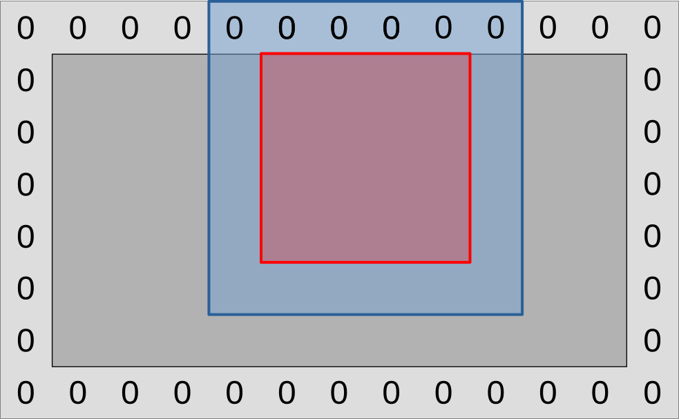
This mapping from work-items to computations has one advantage, which is that GPU work-items work independently of each other. But it has one drawback, which is that work-items perform redundant input loading work. Indeed, most of the inputs that a particular work item loads (blue region) correspond to the central data point (red square) that another work item needs to load.

If we are lucky, the GPU’s cache hierarchy will acknowledge this repeating load pattern and optimize it by turning these slow video RAM accesses into fast cache accesses. But because work item execution is unordered, there is no guarantee that such caching will happen with good efficiency. Especially when one considers that GPU caches are barely larger than their CPU counterpart, while being shared between many more concurrent tasks.

And because GPUs are as memory bandwidth challenged as CPUs, any optimization that has a chance to reduce the amount of memory accesses that are not served by fast local caches and must go all the way to VRAM is worth trying out.

On GPUs, the preferred mechanism for this is shared memory, which lets you reserve a fraction of a compute unit’s cache for the purpose of manually managing it in whatever way you fancy. And in this chapter we will leverage this feature in order to get a stronger guarantee that most input data loads that a workgroup performs go through cache, not VRAM.

Leveraging shared memory

Because GPU shared memory is local to a certain workgroup and GPUs are bad at conditional and irregular logic, the best way to leverage shared memory here is to rethink how we map our simulation work to the GPU’s work-items.

Instead of associating each GPU work-item with one simulation output data point, we are now going to set up workgroups such that each work-item is associated with one input data point:

On the diagram above, a GPU workgroup now maps onto the entire colored region of the simulation domain, red and blue surfaces included.

As this workgroup begins to execute, each of its work-items will proceed to load the (U, V) data point associated with its current location from VRAM, then save it to a shared memory location that every other work-item in the workgroup has access to.

A workgroup barrier will then be used to wait for all work-items to be done. And after this, the work-items within the blue region will be done and exit the compute shader early. Meanwhile, work-items within the red region will proceed to load all their inputs from shared memory, then use these to compute the updated data point associated with their designated input location as before.

If we zoom out from this single workgroup view and try to get a picture of how the entire simulation domain maps into workgroups and work-items, it will look like this:

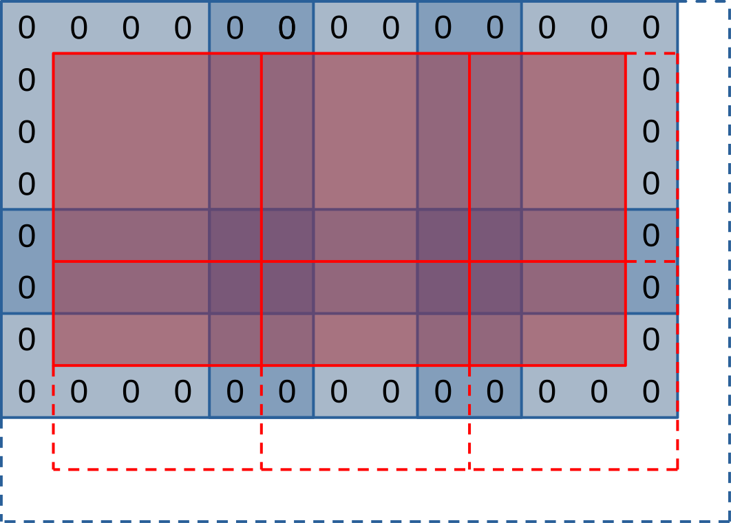
On the diagram above, each workgroup aims to produce a tile of outputs within the simulation domain (red square), and to this end it will first loading a larger set of input values (blue region) into shared memory. Much like in our initial algorithm, workgroups on the right and bottom edges of the simulation domain will extend beyond the end of it (dashed lines) and will need special care to avoid out-of-bounds memory reads and writes.

This picture lets you see that our new use of shared memory does not only come with advantages, but also has some drawbacks:

• The input regions of our work-groups (blue squares) overlap with each other (darker blue regions). This will result in some redundant input loads from VRAM.
• The outermost work-items of our work-groups exit early after loading simulation inputs. This will result in reduced execution efficiency as only a subset of each workgroup will participate in the rest of the computation.

Thankfully, this waste of memory and execution resource only concerns the outermost work-items of each work-group. Therefore, we expect that…

• Workgroups with a larger number of work-items should execute more efficiently, as they have more work-items in the central region and less in the edge region.
• Workgroups with a square-ish aspect ratio should execute more efficiently, as a square shape is mathematically optimal from the perspective of putting more work-items at the center of the workgroup and less on the edges.

But due to the conflicting constraints of GPU hardware (mapping of work-items to SIMD units, memory access granularity, maximal number of resources per workgroup, generation-dependent ability of NVidia hardware to reallocate idle work-items to other workgroups…), the reality is going to be more nuanced than “large square workgroups are better”, and we expect a certain hardware-specific workgroup size to be optimal. It it thus best to keep workgroup size as a tuning parameter that can be adjusted through empirical microbenchmarking, as we have done so far.

First implementation

Before we begin to use shared memory, we must first allocate it. The easiest and most performant way to do so, when available, is to allocate it at GLSL compile time. We can do this here by naming the specialization constants that control our workgroup size…

// In exercises/src/grayscott/common.comp

// This code looks stupid, but alas the rules of GLSL do not allow anything else
layout(local_size_x = 8, local_size_y = 8) in;
layout(local_size_x_id = 0, local_size_y_id = 1) in;
layout(constant_id = 0) const uint WORKGROUP_COLS = 8;
layout(constant_id = 1) const uint WORKGROUP_ROWS = 8;
const uvec2 WORKGROUP_SIZE = uvec2(WORKGROUP_COLS, WORKGROUP_ROWS);

…and allocating a matching amount of shared memory in which we will later store (U, V) values:

// In exercises/src/grayscott/step.comp

// Shared memory for exchanging (U, V) pairs between work-item
shared vec2 uv_cache[WORKGROUP_COLS][WORKGROUP_ROWS];

To make access to this shared memory convenient, we will then add a pair of functions. One lets a work-item store its (U, V) input at its designated location. The other lets a work item load data from shared memory at a certain relative offset with respect to its designated location.

// Save the (U, V) value that this work-item loaded so that the rest of the
// workgroup may later access it efficiently
void set_uv_cache(vec2 uv) {
   uv_cache[gl_LocalInvocationID.x][gl_LocalInvocationID.y] = uv;
}

// Get an (U, V) value that was previously saved by a neighboring work-item
// within this workgroup. Remember to use a barrier() first!
vec2 get_uv_cache(ivec2 offset) {
   const ivec2 shared_pos = ivec2(gl_LocalInvocationID.xy) + offset.xy;
   return uv_cache[shared_pos.x][shared_pos.y];
}

Now that this is done, we must rethink our mapping from GPU work-items to positions within the simulation domain, in order to acknowledge the fact that our work-groups overlap with each other. This concern will be taken care of by another new work_item_pos() GLSL function. And while we are at it, we will also add another is_workgroup_output() function, which tells if our work-item is responsible for producing an output data point.

// Size of the "border" at the edge of work-group, where work-items
// only read inputs and do not write outputs down
const uint BORDER_SIZE = 1;

// Size of the output region of a work-group, accounting for the input border
const uvec2 WORKGROUP_OUTPUT_SIZE = WORKGROUP_SIZE - 2 * uvec2(BORDER_SIZE);

// Truth that this work-item is within the output region of the workgroup
//
// Note that this is a necessary condition for emitting output data, but not a
// sufficient one. work_item_pos() must also fall inside of the output region
// of the simulation dataset, before data_end_pos().
bool is_workgroup_output() {
    const uvec2 OUTPUT_START = uvec2(BORDER_SIZE);
    const uvec2 OUTPUT_END = OUTPUT_START + WORKGROUP_OUTPUT_SIZE;
    const uvec2 item_id = gl_LocalInvocationID.xy;
    return all(greaterThanEqual(item_id, OUTPUT_START))
           && all(lessThan(item_id, OUTPUT_END));
}

// Position of the simulation dataset this work-item should read data from,
// and potentially write data to if it is in the central region of the workgroup
uvec2 work_item_pos() {
   const uvec2 workgroup_topleft = gl_WorkGroupID.xy * WORKGROUP_OUTPUT_SIZE;
   return workgroup_topleft + gl_LocalInvocationID.xy;
}

Given this, we are now ready to rewrite the beginning of our compute shader entry point, where inputs are loaded from VRAM. As before, we begin by finding out which position of our simulation domain our work-item maps into.

void main() {
   // Map work-items into a position within the simulation domain
   const uvec2 pos = work_item_pos();

   // [ ... ]

But after that, we are not allowed to immediately discard work-items which fall out of the simulation domain. Indeed, the barrier() GLSL function, which is used to wait until all work-items are done writing to shared memory, mandates that all work-items within the workgroup be still executing.

We must therefore keep around out of bounds work-items for now, using conditional logic to ensure that they do not perform out-of-bounds memory accesses.

// Load and share our designated (U, V) value, if any
vec2 uv = vec2(0.0);
if (all(lessThan(pos, padded_end_pos()))) {
    uv = read(pos);
    set_uv_cache(uv);
}

After this, we can wait for the workgroup to finish initializing its shared memory cache…

// Wait for the shared (U, V) cache to be ready
barrier();

…and it is only then that we will be able to discard out-of-bounds GPU work-items:

// Discard work-items that are out of bounds for output production work
if (!is_workgroup_output() || any(greaterThanEqual(pos, data_end_pos()))) {
    return;
}

Finally, we can adapt our diffusion gradient computation to use our new shared memory cache…

// Compute the diffusion gradient for U and V
const mat3 weights = stencil_weights();
vec2 full_uv = vec2(0.0);
for (int rel_y = -1; rel_y <= 1; ++rel_y) {
    for (int rel_x = -1; rel_x <= 1; ++rel_x) {
        const vec2 stencil_uv = get_uv_cache(ivec2(rel_x, rel_y));
        const float weight = weights[rel_x + 1][rel_y + 1];
        full_uv += weight * (stencil_uv - uv);
    }
}

…and the rest of the step compute shader GLSL code will not change.

The CPU side of the computation will not change much, but it does need two adjustments, one of the user input validation side and one of the simulation scheduling side.

Our new simulation logic, where workgroups have input-loading edges and an output production center, is incompatible with workgroups that contain less than 3 work-items on either side. We should therefore error out when the user requests such a work-group configuration, and we can do so by adding the following check at the beginning of the Pipelines::new() constructor:

// In exercises/src/grayscott/pipeline.rs

// Error out when an incompatible workgroup size is specified
let pipeline = &options.pipeline;
let check_side = |side: NonZeroU32| side.get() >= 3;
assert!(
    check_side(pipeline.workgroup_cols) && check_side(pipeline.workgroup_rows),
    "GPU workgroups must have at least three work-items in each dimension"
);

The schedule_simulation() function, which schedules the execution of the step compute pipeline, also needs to change, because our mapping from workgroups to simulation domain elements has changed. This is done by adjusting the initial simulate_workgroups computation to add a pair of - 2 that takes the input-loading edges out of the equation:

let dispatch_size = |domain_size: usize, workgroup_size: NonZeroU32| {
    domain_size.div_ceil(workgroup_size.get() as usize - 2) as u32
};
let simulate_workgroups = [
    dispatch_size(options.num_cols, options.pipeline.workgroup_cols),
    dispatch_size(options.num_rows, options.pipeline.workgroup_rows),
    1,
];

First benchmark

Unfortunately, this first implementation of the shared memory optimization does not perform as well as we would hope. Here is its effect on performance on the author’s AMD Radeon 5600M GPU:

run_simulation/workgroup8x8/domain2048x1024/total512/image32/compute
                        time:   [122.48 ms 122.61 ms 122.82 ms]
                        thrpt:  [8.7421 Gelem/s 8.7572 Gelem/s 8.7670 Gelem/s]
                 change:
                        time:   [-5.2863% -3.7811% -2.3117%] (p = 0.00 < 0.05)
                        thrpt:  [+2.3664% +3.9297% +5.5814%]
                        Performance has improved.

run_simulation/workgroup16x8/domain2048x1024/total512/image32/compute
                        time:   [124.89 ms 125.15 ms 125.41 ms]
                        thrpt:  [8.5621 Gelem/s 8.5795 Gelem/s 8.5978 Gelem/s]
                 change:
                        time:   [+21.130% +22.781% +24.736%] (p = 0.00 < 0.05)
                        thrpt:  [-19.831% -18.554% -17.444%]
                        Performance has regressed.

run_simulation/workgroup16x16/domain2048x1024/total512/image32/compute
                        time:   [197.14 ms 197.42 ms 197.68 ms]
                        thrpt:  [5.4318 Gelem/s 5.4388 Gelem/s 5.4466 Gelem/s]
                 change:
                        time:   [+76.474% +79.543% +82.293%] (p = 0.00 < 0.05)
                        thrpt:  [-45.143% -44.303% -43.334%]
                        Performance has regressed.

run_simulation/workgroup32x16/domain2048x1024/total512/image32/compute
                        time:   [192.35 ms 192.78 ms 193.23 ms]
                        thrpt:  [5.5567 Gelem/s 5.5696 Gelem/s 5.5824 Gelem/s]
                 change:
                        time:   [+105.24% +107.32% +109.64%] (p = 0.00 < 0.05)
                        thrpt:  [-52.300% -51.765% -51.277%]
                        Performance has regressed.

run_simulation/workgroup32x32/domain2048x1024/total512/image32/compute
                        time:   [222.67 ms 223.16 ms 223.40 ms]
                        thrpt:  [4.8063 Gelem/s 4.8116 Gelem/s 4.8221 Gelem/s]
                 change:
                        time:   [+124.76% +129.62% +135.86%] (p = 0.00 < 0.05)
                        thrpt:  [-57.602% -56.450% -55.508%]
                        Performance has regressed.

There are two things that are surprising about these results, and not in a good way:

1. We expected use of shared memory to improve our simulation’s performance, or at least not change it much if the GPU cache already knew how to handle the initial logic well. But instead our use of shared memory causes a major performance regression.
2. We expected execution and memory access inefficiencies related to the use of shared memory to have a lower impact on performance as the workgroup size gets larger. But instead the larger our workgroups are, the worse the performance regression gets.

Overall, it looks as if the more intensively we exercised shared memory with a larger workgroup, the more we ran into a severe hardware performance bottleneck related to our use of shared memory. Which begs the question: what could that hardware performance bottleneck be?

Bank conflicts

To answer this question, we need to look into how GPU caches, which shared memory is made of, are organized at the hardware level.

Like any piece of modern computing hardware, GPU caches are accessed via several independent load/store units that can operate in parallel. But sadly the circuitry associated with these load/store units is complex enough that hardware manufacturers cannot afford to provide one load/store unit per accessible memory location of the cache.

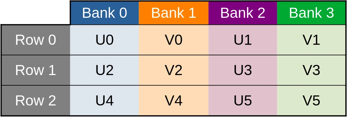
Instead of doing so, manufacturers therefore go for a compromise where some cache accesses can be processed in parallel and others must be serialized. Following an old hardware tradition, load/store units are organized such that memory accesses that target consecutive memory location are faster, and this is how we get the banked cache organization illustrated below:

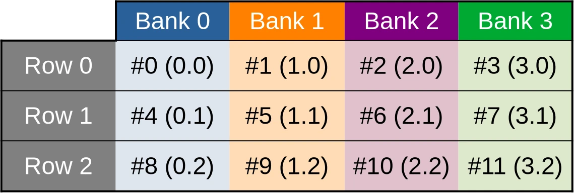
The toy cache example from this illustration possesses 4 independent storage banks (colored table columns), each of which controls 3 data storage cells (table rows). Memory addresses (denoted #N in the diagram) are then distributed across these storage cells in such a way that the first accessible address belongs to the first bank, the second location belongs to the second bank, and so on until we run out of banks. Then we start over at the first bank.

This storage layout ensures that if work is distributed across GPU work-items in such a way that the first work item processes the first shared memory location, the second work item processes the second shared memory location, and so on, then all cache banks will end up being evenly utilized, leading to maximal memory access parallelism and thus maximal performance.

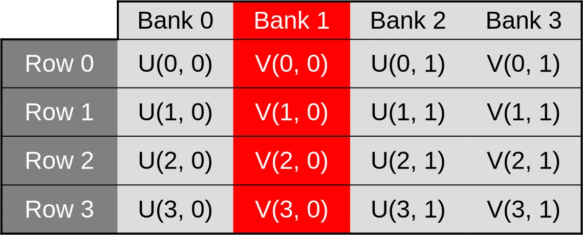
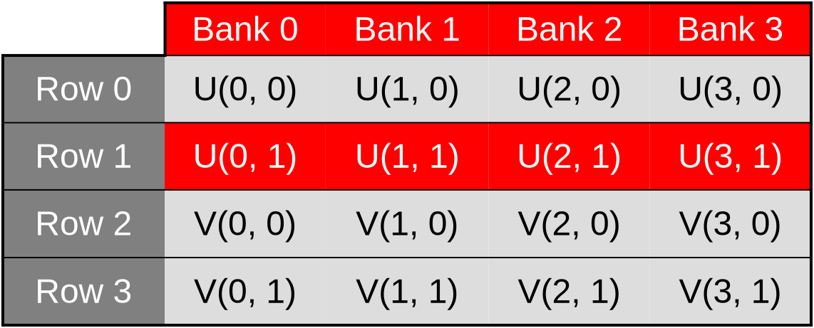
However, things only work out so well as long as cached data are made of primitive 32-bit GPU data atoms. And as you may recall, this is not the case of our current shared memory cache, which is composed of two-dimensional vectors of such data:

// Shared memory for exchanging (U, V) pairs between work-item
shared vec2 uv_cache[WORKGROUP_COLS][WORKGROUP_ROWS];

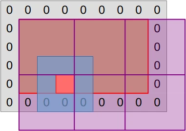
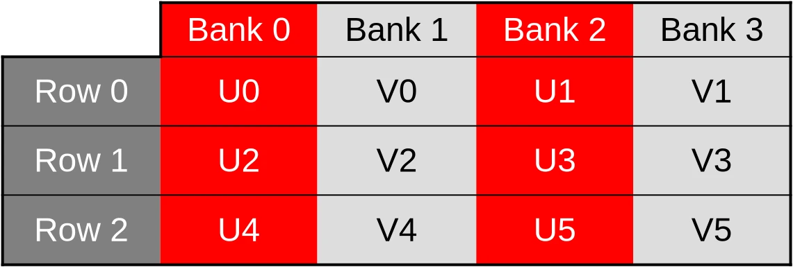
Because of this, our (U, V) data cache ends up being organized in the following manner…

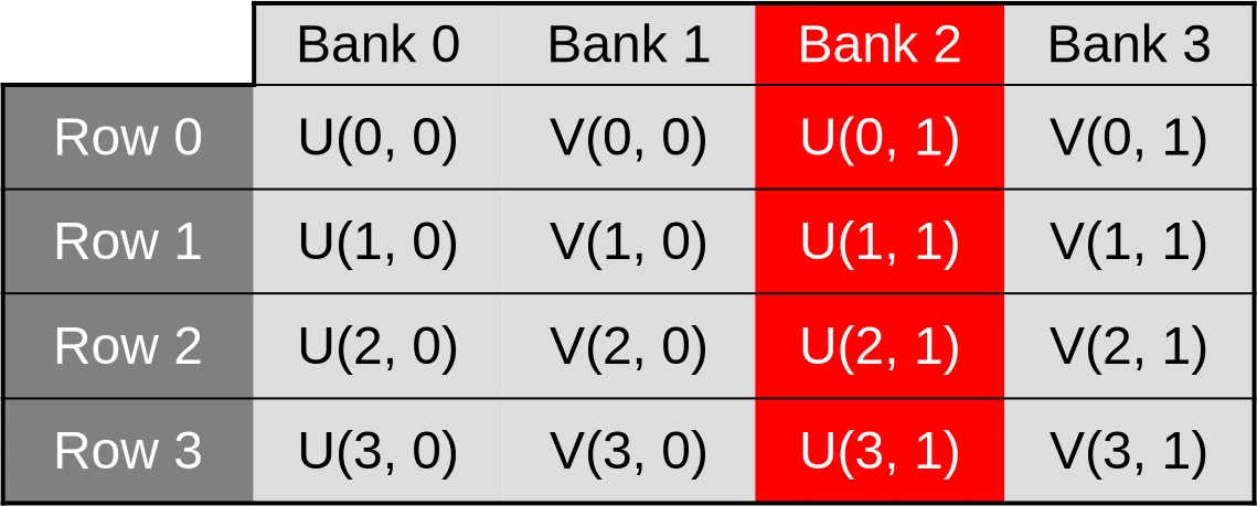
…which means that when the U component of the dataset is accessed via a first 32-bit memory load/store instruction, only one half of the cache banks end up being used…

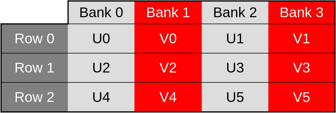
…and when the V component of the dataset later ends up being accessed by a second 32-bit memory load/store instruction, only the other half of the cache banks ends up being used.

It gets worse than that, however. Our shared memory cache is also layed out as a two dimensional array where columns of data are contiguous in memory and rows of data are not.

This is a problem because in computer graphics, 2D images are conventionally layed out in memory such that rows of data are contiguous in memory, and columns are not. And because contiguous memory accesses are more efficient, GPUs normally optimize for this common case by distributing work-items over SIMD units in such a way that work-items on the same row (same Y coordinate, consecutive X coordinates) end up being allocated to the same SIMD unit and processed together.

In our shared memory cache, the data associated with those work-items ends up being stored inside of storage cells whose memory locations are separated by 2 * WORKGROUP_ROWS 32-bit elements. And when WORKGROUP_ROWS is large enough and a power of two, this number is likely to end up being a multiple of the number of cache memory data banks.

We will then end up with worst-case scenarios where cache bank parallelism is extremely under-utilized and all memory accesses from a given hardware SIMD instruction end up being sequentially processed by the same cache bank. For example, accesses to the U coordinate of the first row of data could be processed by the first cache bank…

…accesses to the V coordinate of the first row could be processed by the second bank…

…accesses to the U coordinate of the second row could be processed by the third bank…

…and so on. This scenario, where cache bandwidth is under-utilized because memory accesses that could be processed in parallel are processed sequentially instead, is called a cache bank conflict.

Avoiding bank conflicts

While GPU cache bank conflicts can have a serious impact on runtime performance, they are thankfully easy to resolve once identified.

All we need to do here is to…

• Switch from our former “array-of-structs” data layout, where uv_cache is an array of two-dimensional vectors of data, to an alternate “struct-of-arrays” data layout where uv_cache begins with U concentration data and ends with V concentration data.
• Flip the 2D array axes so that work-items with consecutive X coordinates end up accessing shared memory locations with consecutive memory addresses.

In terms of code, it looks like this:

// Shared memory for exchanging (U, V) pairs between work-item
shared float uv_cache[2][WORKGROUP_ROWS][WORKGROUP_COLS];

// Save the (U, V) value that this work-item loaded so that the rest of the
// workgroup may later access it efficiently
void set_uv_cache(vec2 uv) {
   uv_cache[U][gl_LocalInvocationID.y][gl_LocalInvocationID.x] = uv.x;
   uv_cache[V][gl_LocalInvocationID.y][gl_LocalInvocationID.x] = uv.y;
}

// Get an (U, V) value that was previously saved by a neighboring work-item
// within this workgroup. Remember to use a barrier() first!
vec2 get_uv_cache(ivec2 offset) {
   const ivec2 shared_pos = ivec2(gl_LocalInvocationID.xy) + offset.xy;
   return vec2(
        uv_cache[U][shared_pos.y][shared_pos.x],
        uv_cache[V][shared_pos.y][shared_pos.x]
    );
}

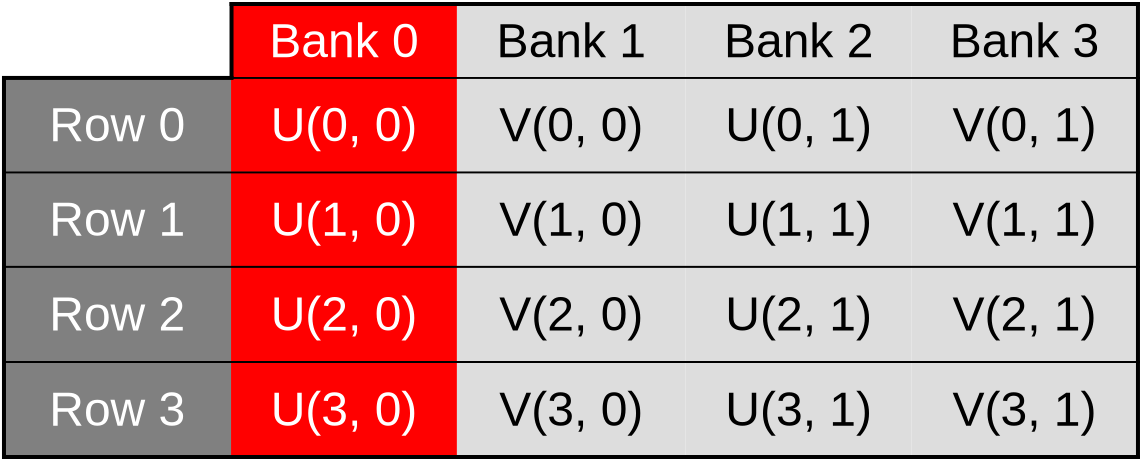
After applying this simple data layout transform, our (U, V) data cache will end up being organized in the following manner…

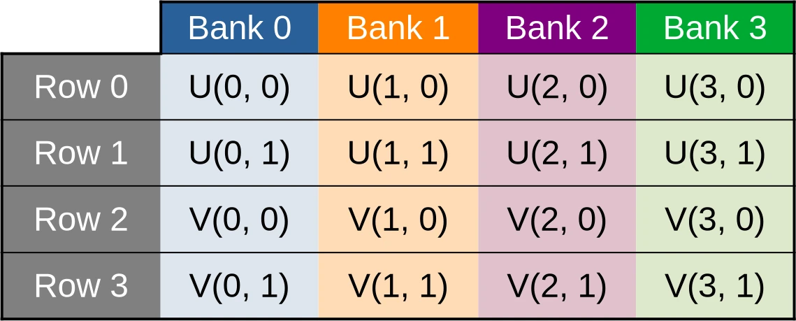
…where data points associated with the U species concentration for the first row of data are contiguous, and thus evenly spread across banks…

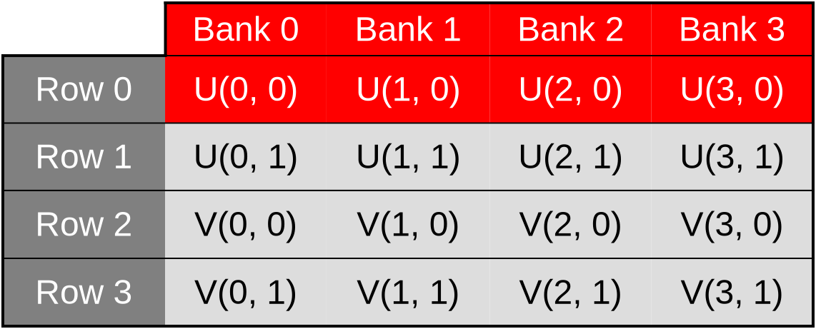
…and this remains true as we switch across rows, access the V species’ concentration, etc.

Because of this, we expect our new shared memory layout to result in a significant performance improvement, where individual shared memory accesses are sped up by up to 2x. Which will have a smaller, but hopefully still significant impact on the performance of the overall simulation.

Exercise

Implement this optimization and measure its performance impact on your hardware.

The improved shared memory layout that avoids bank conflicts should provide a net performance improvement over the original array-of-structs memory layout. But when comparing to the previous chapter, the performance tradeoff of manually managing a shared memory cache vs letting the GPU’s cache do this job is intrinsically hardware-dependent.

So don’t be disappointed if it turns out that on your GPU, using shared memory is not worthwhile even when cache bank conflicts are taken out of the equation.