Introduction

Welcome to this course about high-performance numerical computing with Rust on GPU!

This course builds upon the companion course on CPU computing, and is meant to directly follow it. Basic concepts of the Rust programming language will therefore not be introduced again. Instead, we will see how these concepts can be leveraged to build high-performance GPU computations, using the Vulkan API via the vulkano high-level Rust binding.

These are rather uncommon technological choices in scientific computing, so you may wonder why they were chosen. Rust ecosystem support aside, Vulkan was picked as one of few GPU APIs that manage to avoid the classic design flaws of HPC-centric GPU APIs:

• Numerical computations should aim for maximal portability by default. Nonportable programs are the open-air landfills of HPC: they may seem initially convenient, but come with huge hidden costs and leave major concerns up to future generations.¹
• CPU/GPU performance portability doesn’t work. Decades of research have produced nothing but oversized frameworks of mind-boggling complexity where either CPU or GPU performance does not even remotely match that of well-optimized code on non-toy programs. A GPU-first API can be conceptually simpler, more reliable, and ease optimization; all this saves enough time to let you write a good CPU version of your computational kernel if you need one.
• Proprietary API emulation or imitation doesn’t work. Because the monopoly manufacturer controls the API and has much greater software development resources, all other hardware will always be a second-class citizen with lagging support, unstable runtimes, and poor support of advanced hardware features that the monopoly manufacturer didn’t implement.
• Relying on hardware manufacturer good will doesn’t work. Monopoly manufacturers will not help you write code that works on other hardware, and minority hardware manufacturers have little resources to dedicate to obscure HPC portability technologies with low adoption. It is more effective to force the manufacturers’ hand by basing your work on a widely adopted technology whose reach extends far beyond the relatively small HPC community.

As for the vulkano Rust binding specifically, the choice came down to general maturity, maintenance status, broad Vulkan API coverage, high-quality documentation, ease of installation and good alignment with the Rust design goals of making code type/memory/thread-safe by default.

Pedagogical advice given in the introduction of the CPU course still applies:

• This course is meant to be followed in order, environment setup section aside. Each sections will build upon the concepts taught and the exercise work done in earlier sections.
• The material is written to allow further self-study after the school, so it’s okay to fall a little behind the group. Good understanding is more important than full chapter coverage.
• Solutions to some exercises are provided in the top commits of the solution branch of the repository. To keep the course material maintainable, these only cover exercises where there is one obvious solution, not open-ended problems where you could go down many paths.

As in the CPU course, you can navigate between the course’s sections using several tools:

• The left-hand sidebar, which provides direct access to every page.
  • If your browser window is thin, the sidebar may be hidden by default. In that case you can open (and later close) it using the top-left “triple dash” button.
• The left/right arrow buttons at the end of each page, or your keyboard’s arrow keys.

1. Problems linked to nonportable code include lack of future computation reproducibility, exploding hardware costs, reduced hardware innovation, and ecosystem fragility against unforeseen changes of politics like the ongoing race to the bottom in computational precision. ↩

Environment setup

The development environment for this course will largely extend that of the CPU course. You should therefore begin by following the environment setup process for the CPU course if you have not done so already, including the final test which makes sure that your Rust development environment does work as expected for CPU programming purposes.

Once this is done, we will proceed to extend this CPU development environment into a GPU development environment by going through the following steps:

• Try to make your GPU(s) available for Vulkan development. This is the hardest part, but if this step fails it’s not the end of the world, we can use a GPU emulator instead.
• Add Vulkan development tools to your Rust development environment.
• Download and unpack this course’s version of the exercises/ source code.
• Test that the resulting setup is complete by running some of the course’s code examples.

Host GPU setup

Before a Vulkan-based program can use your GPU, a few system preparations are needed:

• Vulkan relies on GPU hardware features that were introduced around 2012. If your system’s GPUs are older than this, then you will almost certainly need to use a GPU emulator, and can ignore everything else that is said inside of this chapter.
• Doing any kind of work with a GPU requires a working GPU driver. Which, for some popular brands of GPUs, may unfortunately require some work.
• Doing Vulkan work specifically additionally requires a Vulkan implementation that knows how to communicate with your GPU driver.
  • Some GPU drivers provide their own Vulkan implementation. This is common on Windows, but also seen in e.g. NVidia’s Linux drivers.
  • Other GPU drivers expose a standardized interface that a third-party Vulkan implementations can tap into. This is the norm on Linux on macOS.

It is important to point out that you will also need these preparations when using Linux containers, because the containers do not acquire full control of the GPU hardware. They need to go through the host system’s GPU driver, which must therefore be working.

In fact, as a word of warning, containerized setups will likely make it harder for you to get a working GPU setup.¹ Given the option to do so, you should prefer using a native development environment for this course, or any other kind of coding that involves GPUs for that matter.

GPU driver

The procedure for getting a working GPU driver is, as you may imagine, fairly system-dependent. Please select your operating system using the tabs below:

After performing any setup step described above and rebooting, your system should have a working GPU driver. But owing to the highly system-specific nature of this step, we unfortunately won’t yet be able to check this in an OS-agnostic manner. To do that, we will install another component that you are likely to need for this course, namely a Vulkan implementation.

Vulkan implementation

As mentioned above, your GPU driver may or may not come with a Vulkan implementation. If that is not the case, we will want to install one.

Given this preparation, your system should now be ready to run Vulkan apps that use your GPU. How do we know for sure, however? A test app will come in handy here.

Final check

The best way to check if your Vulkan setup works is to run a Vulkan application that can display a list of available devices and make sure that your GPUs are featured in that list.

The Khronos Group, which maintains the Vulkan specification, provide a simple tool for this in the form of the vulkaninfo app, which prints a list of all available devices along with their properties. And for once, planets have aligned properly and all package managers in common use have agreed to name the package that contains this app identically. No matter if you use a Linux distribution’s built-in package manager, brew for macOS, or vcpkg for Windows, the package that contains this utility is called vulkan-tools on every system that the author could think about.

There is just one problem: Vulkan devices have many properties, which means that the default level of detail displayed by vulkaninfo is unbrearable. For example, it emits more than 6000 lines of textual output on the author’s laptop at the time of writing.

Thankfully there is an easy fix for that: add the --summary command line option, and you will get a reasonably concise device list at the end of the output. Here’s the output from the author’s laptop:

vulkaninfo --summary

[ ... global Vulkan implementation properties ... ]

Devices:
========
GPU0:
        apiVersion         = 1.4.311
        driverVersion      = 25.1.4
        vendorID           = 0x1002
        deviceID           = 0x1636
        deviceType         = PHYSICAL_DEVICE_TYPE_INTEGRATED_GPU
        deviceName         = AMD Radeon Graphics (RADV RENOIR)
        driverID           = DRIVER_ID_MESA_RADV
        driverName         = radv
        driverInfo         = Mesa 25.1.4-arch1.1
        conformanceVersion = 1.4.0.0
        deviceUUID         = 00000000-0800-0000-0000-000000000000
        driverUUID         = 414d442d-4d45-5341-2d44-525600000000
GPU1:
        apiVersion         = 1.4.311
        driverVersion      = 25.1.4
        vendorID           = 0x1002
        deviceID           = 0x731f
        deviceType         = PHYSICAL_DEVICE_TYPE_DISCRETE_GPU
        deviceName         = AMD Radeon RX 5600M (RADV NAVI10)
        driverID           = DRIVER_ID_MESA_RADV
        driverName         = radv
        driverInfo         = Mesa 25.1.4-arch1.1
        conformanceVersion = 1.4.0.0
        deviceUUID         = 00000000-0300-0000-0000-000000000000
        driverUUID         = 414d442d-4d45-5341-2d44-525600000000
GPU2:
        apiVersion         = 1.4.311
        driverVersion      = 25.1.4
        vendorID           = 0x10005
        deviceID           = 0x0000
        deviceType         = PHYSICAL_DEVICE_TYPE_CPU
        deviceName         = llvmpipe (LLVM 20.1.6, 256 bits)
        driverID           = DRIVER_ID_MESA_LLVMPIPE
        driverName         = llvmpipe
        driverInfo         = Mesa 25.1.4-arch1.1 (LLVM 20.1.6)
        conformanceVersion = 1.3.1.1
        deviceUUID         = 6d657361-3235-2e31-2e34-2d6172636800
        driverUUID         = 6c6c766d-7069-7065-5555-494400000000

As you can see, this particular system has three Vulkan devices available:

• An AMD GPU that’s integrated into the same package as the CPU (low-power, low-performance)
• Another AMD GPU that is separated from the CPU aka discrete (high-power, high-performance)
• A GPU emulator called llvmpipe that is useful for debugging, and as a fallback for systems where there is no easy way to get a real hardware GPU to work (e.g. continuous integration of software hosted on GitHub or GitLab).

If you see all the Vulkan devices that you expect in the output of this command, that’s great! You are done with this chapter and can move to the next one. Otherwise, please go through this page’s instructions slowly again, making sure that you have not forgotten anything, and if not ping the teacher and we’ll try to figure it out together.

1. In addition to a working GPU driver on the host sytem and a working Vulkan stack inside of the container, you need to have working communication between the two. This assumes that they are compatible, which is anything but a given when e.g. running Linux containers on Windows or macOS. It also doesn’t help that most container runtimes are designed to operate as a black box (with few ways for users to observe and control the inner machinery) and attempt to sandbox containers (which may prevent them from getting access to the host GPU in the default container runtime configuration). ↩

2. Unless you are using an exotic configuration like an old macOS release running on a recent computer, that is, but if you know how to get yourself into this sort of Apple-unsupported configuration, we trust you to also know how to keep its GPU driver working… :) ↩

3. NVidia’s GPU drivers have historically tapped into unstable APIs of the Linux kernel that may change across even bugfix kernel releases, and this makes them highly vulnerable to breakage across system updates. To make matters worse, their software license would also prevent Linux distributions from shipping these drivers into their official software repository, which prevented distributions from enforcing kernel/driver compatibility at the package manager level. The situation has recently improved for newer hardware (>= Turing generation), where a new “open-source driver” (actually a thin open-source layer over an enormous encrypted+signed binary blob running on a hidden RISC-V CPU because this is NVidia) has been released with a license that enables distributions to ship it as a normal package. ↩

4. The unfortunate popularity of “stable” distributions like Red Hat Enterprise or Ubuntu LTS, which take pride in embalming ancient software releases and wasting thousands of developer hours into backporting bugfixes from newer releases, make this harder than it should be. But when an old kernel gets in the way of hardware support and a full distribution upgrade is not an option, consider upgrading the kernel alone using facilities like Ubuntu’s “HardWare Enablement” (-hwe) kernel packages. ↩

Development tools

The Rust development environment that was set up for the CPU computing course contains many things that are also needed for this GPU computing course too. But we are also going to need a few other things that are specific to this course. To be more specific…

• If you previously used containers, you must first switch to another container (based on the CPU one) that features Vulkan development tools. Then you can adjust your container’s execution configuration to expose host GPUs to the containerized Linux system.
  • In the 2025 edition, it was reported that Windows and macOS container runtimes like Docker Desktop struggle with exposing GPU hardware from the host to the container. Users of these operating systems should either favor native installations or accept potentially getting stuck with a GPU emulation.
• If you previously performed a native installation, then you must install Vulkan development tools alongside the Rust development tools that you already have.

Linux containers

Switching to the new source code

As you may remember, when setting up your container for the CPU course, you started by downloading and unpacking an archive which contains a source code directory called exercises/.

We will do mostly the same for this course, but the source code will obviously be different. Therefore, please rename your previous exercises directory to something else (or switch to a different parent directory), then follow the following instructions.

if [ -e exercises ]; then
    echo "ERROR: Please move or delete the existing 'exercises' subdirectory"
else
    curl -LO https://numerical-rust-gpu-96deb7.pages.in2p3.fr/setup/exercises.zip  \
    && unzip exercises.zip  \
    && rm exercises.zip
fi

Invoke-Command -ScriptBlock {
      $ErrorActionPreference="Stop"
      if (Test-Path exercises) {
            throw "ERROR: Please move or delete the existing 'exercises' subdirectory"
      }
      Invoke-WebRequest https://numerical-rust-gpu-96deb7.pages.in2p3.fr/setup/exercises.zip  `
                        -OutFile exercises.zip
      Expand-Archive exercises.zip -DestinationPath .
      Remove-Item exercises.zip
}

Switching to the GPU image

During the CPU course, you have used a container image with a name that has numerical-rust-cpu in it, such as gitlab-registry.in2p3.fr/grasland/numerical-rust-cpu/rust_light:latest. It is now time to switch to another version of this image that has GPU tooling built into it.

• If you used the image directly, that’s easy, just replace cpu with gpu in the image name and all associated container execution commands that you use. In the above example, you would switch gitlab-registry.in2p3.fr/grasland/numerical-rust-gpu/rust_light:latest.
• If you built a container image of your own on top of the course’s image, then you will have a bit more work to do, in the form of replaying your changes on top of your new images. Which shouldn’t be too hard either… if you used a proper Dockerfile instead of raw docker commit.

But unfortunately, that’s not the end of it. Try to run vulkaninfo --summary inside of the resulting container, and you will likely figure out that some of your host GPUs are likely not visible inside of the container. If that’s the case, then I have bad news for you: you have some system-specific work to do if you want to be able to use your GPUs inside of the container.

Exposing host GPUs

Please click the following tab that best describes your host system for further guidance:

--gpus=all --env VK_ICD_FILENAMES=/usr/share/glvnd/egl_vendor.d/10_nvidia.json

--nv --env VK_ICD_FILENAMES=/usr/share/glvnd/egl_vendor.d/10_nvidia.json

New command line arguments and container image name aside, the procedure for starting up a container will be mostly identical to that used for the CPU course. So you will want to get back to the appropriate section of the CPU course’s container setup instructions and follow the instructions for your container and system configuration again.

Once that is done, please run vulkaninfo --summary inside of a shell within the container and check that the Vulkan device list matches what you get on the host, driver version details aside.

Testing your setup

Your Rust development environment should now be ready for this course’s practical work. I strongly advise testing it by running the following script:

curl -LO https://gitlab.in2p3.fr/grasland/numerical-rust-gpu/-/archive/solution/numerical-rust-gpu-solution.zip  \
&& unzip numerical-rust-gpu-solution.zip  \
&& rm numerical-rust-gpu-solution.zip  \
&& cd numerical-rust-gpu-solution/exercises  \
&& echo "------"  \
&& cargo run --release --bin info -- -p  \
&& echo "------"  \
&& cargo run --release --bin square -- -p  \
&& cd ../..  \
&& rm -rf numerical-rust-gpu-solution

It performs the following actions, whose outcome should be manually checked:

• Run a Rust program that should produce the same device list as vulkaninfo --summary. This tells you that any device that gets correctly detected by a C Vulkan program also gets correctly detected by a Rust Vulkan program, as one would expect.
• Run another program that uses a simple heuristic to pick the Vulkan device that should be most performant, then uses that device to square an array of floating-point numbers, then checks the results. You should make sure the device selection that this program made is sensible and its final result check passed.
• If everything went well, the script will clean up after itself by deleting all previously created files.

Native installation

While containers are often lauded for making it easier to reproduce someone else’s development environment on your machine, GPUs actually invert this rule of thumb. As soon GPUs get involved, it’s often easier to get something working with a native installation.

The reason why that is the case is that before we get any chance of having a working GPU setup inside of a container, we must first get a working GPU setup on the host system. And once you have taken care of that (which is often the hardest part), getting the rest of a native development environment up and running is not that much extra work.

As before, we will will assume that you have already taken care of setting up a native development environment for Rust CPU development, and this documentation will therefore only focus on the changes needed to get this setup ready for native Vulkan development. Which will basically boil down to installing a couple of Vulkan development tools.

Vulkan validation layers

Vulkan came in a context where GPU applications were often bottlenecked by API overheads, and one of its central design goals was to improve upon that. A particularly controversial decision taken then was to remove mandatory parameter validation from the API, instead making it undefined behavior to pass any kind of unexpected parameter value to a Vulkan function.

This may be amazing for run-time performance, but certainly does not result in a great application development experience. Therefore it was also made possible to bring such checks back as an optional “validation” layer, that is meant to be used during application development and later removed in production. As a bonus, because this layer was only meant for development purposes and operated under no performance constraint, it could also…

• Perform checks that are much more detailed than those that any GPU API performed before, finding more errors in GPU-side code and CPU-GPU synchronization patterns.
• Supplement API usage error reporting with more opinionated “best practices” and “performance” lints that are more similar to compiler warnings in spirit.

Because this package is meant to be used for development purposes, it is not a default part of Vulkan installations. Thankfully, all commonly used systems have a package for that:

• Debian/Ubuntu/openSUSE/Brew: vulkan-validationlayers
• Arch/Fedora/RHEL: vulkan-validation-layers
• Windows: Best installed as part of the LunarG Vulkan SDK

shaderc

Older GPU APIs relied on GPU drivers to implement a compiler for a C-like language, which proved to be a bad idea as GPU manufacturers are terrible compiler developers (and terrible software developers in general). Applications thus experienced constant issues linked to those compilers, from uneven performance across hardware to incorrect run-time program behavior.

To get rid of this pain, Vulkan has switched to an AoT/JiT hybrid compilation model where GPU code is first compiled into a simplified assembly-like interpreted representation called SPIR-V on the developer’s machine, and it is this intermediate representation that gets sent to the GPU driver for final compilation into a device- and driver-specific binary.

Because of this, our development setup is going to require a compiler that goes from the GLSL domain-specific language (which is a common choice for GPU code, we’ll get into why during the course) to SPIR-V. The vulkano Rust binding that we use is specifically designed to use shaderc, which is a compiler that is maintained by the Android development team.

Unfortunately, shaderc is not packaged by all Linux distributions. You may therefore need to either use the official binaries or build it from source. In the latter case, you are going to need…

• CMake
• Ninja
• C and C++ compilers
• Python
• git

…and once those dependencies are available, you should be able to build and install the latest upstream-tested version of shaderc and its dependencies using the following script:

git clone --branch=known-good https://github.com/google/shaderc  \
&& cd shaderc  \
&& ./update_shaderc_sources.py  \
&& cd src  \
&& ./utils/git-sync-deps  \
&& mkdir build  \
&& cd build  \
&& cmake -GNinja -DCMAKE_BUILD_TYPE=Release ..  \
&& ninja  \
&& ctest -j$(nproc)  \
&& sudo ninja install  \
&& cd ../../..  \
&& rm -rf shaderc

Whether you download binaries or build from source, the resulting shaderc installation location will likely not be in the default search path of the associated shaderc-sys Rust bindings. We will want to fix this, otherwise the bindings will try to be helpful by automatically downloading and building an internal copy of shaderc insternally. This may fail if the dependencies are not available, and is otherwise inefficient as such a build will need to be performed once per project that uses shaderc-sys and again if the build directory is ever discarded using something like cargo clean.

To point shaderc-sys in the right direction, find the directory in which the libshaderc_combined static library was installed (typically some variation of /usr/local/lib when building from source on Unix systems). Then adjust your Rust development environment’s configuration so that the SHADERC_LIB_DIR environment variable is set to point to this directory.

Syntax highlighting

For an optimal GPU development experience, you will want to set up your code editor to apply GLSL syntax highlighting to files with a .comp extension. In the case of Visual Studio Code, this can be done by installing the slevesque.shader extension.

Testing your setup

Your Rust development environment should now be ready for this course’s practical work. I strongly advise testing it by running the following script:

curl -LO https://gitlab.in2p3.fr/grasland/numerical-rust-gpu/-/archive/solution/numerical-rust-gpu-solution.zip  \
&& unzip numerical-rust-gpu-solution.zip  \
&& rm numerical-rust-gpu-solution.zip  \
&& cd numerical-rust-gpu-solution/exercises  \
&& echo "------"  \
&& cargo run --release --bin info -- -p  \
&& echo "------"  \
&& cargo run --release --bin square -- -p  \
&& cd ../..  \
&& rm -rf numerical-rust-gpu-solution

Invoke-Command -ScriptBlock {
      $ErrorActionPreference="Stop"

      Invoke-WebRequest https://gitlab.in2p3.fr/grasland/numerical-rust-gpu/-/archive/solution/numerical-rust-gpu-solution.zip  `
                        -OutFile solution.zip
      Expand-Archive solution.zip -DestinationPath .
      Remove-Item solution.zip
      Set-Location numerical-rust-gpu-solution/exercises

      Write-Output "------"
      cargo run --release --bin info -- -p

      Write-Output "------"
      cargo run --release --bin square -- -p

      Set-Location ..\..
      Remove-Item numerical-rust-gpu-solution -Recurse
}

It performs the following actions, whose outcome should be manually checked:

• Run a Rust program that should produce the same device list as vulkaninfo --summary. This tells you that any device that gets correctly detected by a C Vulkan program also gets correctly detected by a Rust Vulkan program, as one would expect.
• Run another program that uses a simple heuristic to pick the Vulkan device that should be most performant, then uses that device to square an array of floating-point numbers, then checks the results. You should make sure the device selection that this program made is sensible and its final result check passed.
• If everything went well, the script will clean up after itself by deleting all previously created files.

Training-day instructions

Expectations and conventions

Welcome to this practical about high-performance GPU computing in Rust!

This course is meant to follow the previous one, which is about CPU computing. It is assumed that you have followed that course, and therefore we will not repeat anything that was said there. However, if your memory is hazy and you are unsure about what a particular construct in the Rust code examples does, please ping the teacher for guidance.

Although some familiarity with Rust CPU programming is assumed, no particular GPU programming knowledge is expected beyond basic knowledge of GPU hardware architecture. Indeed, the GPU API that we will use (Vulkan) is different enough from other (CUDA- or OpenMP-like) APIs that are more commonly used in HPC that knowledge of those APIs may cause extra confusion. The course’s introduction explains why we are using Vulkan and not these other APIs like everyone else.

Exercises source code

At the time where you registered, you should have been directed to instructions for setting up your development environment. If you did not follow these instructions yet, this is the right time!

Now that the course has begun, we will download a up-to-date copy of the exercises’ source code and unpack it somewhere inside of your development environement. This will create a subdirectory called exercises/ in which we will be working during the rest of the course.

Please pick your environement below in order to get appropriate instructions:

cd ~
# Can't use rm -rf exercises because we must keep the bind mount alive
for f in $(ls -A exercises); do rm -rf exercises/$f; done  \
&& curl -LO https://numerical-rust-gpu-96deb7.pages.in2p3.fr/setup/exercises.zip  \
&& unzip -u exercises.zip  \
&& rm exercises.zip  \
&& cd exercises

Invoke-Command -ScriptBlock {
      $ErrorActionPreference="Stop"
      if (Test-Path exercises) {
            throw "ERROR: Please move or delete the existing 'exercises' subdirectory"
      }
      Invoke-WebRequest https://numerical-rust-cpu-96deb7.pages.in2p3.fr/setup/exercises.zip  `
                        -OutFile exercises.zip
      Expand-Archive exercises.zip -DestinationPath .
      Remove-Item exercises.zip
      Set-Location exercises
}

if [ -e exercises ]; then
    echo "ERROR: Please move or delete the existing 'exercises' subdirectory"
else
    curl -LO https://numerical-rust-gpu-96deb7.pages.in2p3.fr/setup/exercises.zip  \
    && unzip exercises.zip  \
    && rm exercises.zip  \
    && cd exercises
fi

General advice

Some exercises are based on code examples that are purposely incorrect. Therefore, if some code fails to build, it may not come from a mistake of the course author, but from some missing work on your side. The course material should explicitly point out when that is the case.

If you encounter any failure which does not seem expected, or if you otherwise get stuck, please call the trainer for guidance!

With that being said, let’s get started with actual Rust code. You can move to the next page, or any other page within the course for that matter, through the following means:

• Left and right keyboard arrow keys will switch to the previous/next page. Equivalently, arrow buttons will be displayed at the end of each page, doing the same thing.
• There is a menu on the left (not shown by default on small screen, use the top-left button to show it) that allows you to quickly jump to any page of the course. Note, however, that the course material is designed to be read in order.
• With the magnifying glass icon in the top-left corner, or the “S” keyboard shortcut, you can open a search bar that lets you look up content by keywords.

1. If you’re using rust_code_server, this means using the terminal pane of the web-based VSCode editor. ↩

2. That would be a regular shell for a local Linux/macOS installation and a Windows Subsystem for Linux shell for WSL. ↩

Instance

Any API that lets developers interact with a complex system must strike a balance between flexibility and ease of use. Vulkan goes unusually far on the flexibility side of this tradeoff by providing you with many tuning knobs at every stage of an execution process that most other GPU APIs largely hide from you. It therefore requires you to acquire an unusually good understanding of the complex process through which a GPU-based program gets things done.

In the first part of this course, we will make this complexity tractable by introducing it piece-wise, in the context of a trivial GPU program that merely squares an array of floating-point numbers. In the second part of the course, you will then see that once these basic concepts of Vulkan are understood, they easily scale them up to the complexity of a full Gray-Scott reaction.

As a first step, this chapter will cover how you can load the Vulkan library from Rust, set up a Vulkan instance in a way that eases later debugging, and enumerate available Vulkan devices.

Introducing vulkano

The first step that we must take before we can use Vulkan in Rust code, is to link your program to a Vulkan binding. This is a Rust crate that handles the hard work of linking to the Vulkan C library and exposing a Rust layer on top of it so that your Rust code may interact with it.

In this course, we will use the vulkano crate for this purpose. This crate builds on top of the auto-generated ash crate, which closely matches the Vulkan C API with only minor Rust-specific API tweaks, by supplementing it with two layers of abstraction:

• A low-level layer that re-exposes Vulkan types and functions in a manner that is more in line with Rust programmer expectations. For example, C-style free functions that operate on their first pointer parameter are replaced with Rust-style structs with methods.
• A high-level layer that automates away some common operations (like sub-allocation of GPU memory allocations into smaller chunks) and makes as many operations as possible safe (no possibility for undefined behavior).

Crucially, this layering is fine-grained (done individually for each Vulkan object type) and transparent (any high-level object lets you access the lower-level object below it). As a result, if you ever encounter a situation where the high-level layer has made design choices that are not right for your use case, you are always able to drop down to a lower-level layer and do things your own way.

This means that anything you can do with raw Vulkan API calls, you can also do with vulkano. But vulkano will usually give you an alternate way to do things that is easier, fast/flexible enough for most purposes, and requires a lot less unsafe Rust code that must be carefully audited for memory/thread/type safety. For many applications, this is a better tradeoff than using ash directly.

The vulkano dependency has already been added to this course’s example code, but for reference, this is how you would add it:

# You do not need to type in this command, it has already been done for you
cargo add --no-default-features --features=macros vulkano

This adds the vulkano dependency in a manner that disables the x11 feature that enables X11 support. This feature is not needed for this course, where we are not rendering images to X11 windows. And it won’t work in this course’s Linux containers, which do not contain a complete X11 stack as this would unnecessarily increase download size.

We do, however, keep the macros features on, because we will need it in order to use the vulkano-shaders crate later on. We’ll discuss what this crate does and why we need it in a future chapter.

Loading the library

Now that we have the vulkano binding available, we can use it to load the Vulkan library. In principle, you could customize this loading process to e.g. switch between different Vulkan libraries, but in practice this is rarely needed because as we will see later Vulkan provides several tools to customize the behavior of the library.

Hence, for the purpose of this course, we will stick with the default vulkano library-loading method, which is appropriate for almost every Vulkan application:

use std::error::Error;
use vulkano::library::VulkanLibrary;

// Simplify error handling with type-erased errors
type Result<T> = std::result::Result<T, Box<dyn Error>>;

fn main() -> Result<()> {
    // Load the Vulkan library
    let library = VulkanLibrary::new()?;

    // ...

    Ok(())
}

Like all system operations, loading the library can fail if e.g. no Vulkan implementation is installed on the host system, and we need to handle that.

Here, we choose to do it the easy way by converting the associated error type into a type-erased Box<dyn Error> type that can hold all error types, and bubbling this error out of the main() function using the ? error propagation operator. The Rust runtime will then take care of displaying the error message and aborting the program with a nonzero exit code. This basic error handling strategy is good enough for the simple utilities that we will be building throughout this course.

Once errors are handled, we may query the resulting VulkanLibrary object. For example, we can…

• Check which revision of the Vulkan specification is supported. This versioning allows the Vulkan specification to evolve by telling us which newer features can be used by our application.
• Check which Vulkan extensions are supported. Extensions allow Vulkan to support features that do not make sense on every single system supported by the API, such as the ability to display visuals in X11 and Wayland windows on Linux.
• Check which Vulkan layers are available. Layers are stackable plugins that customize the behavior of your Vulkan library without replacing it. For example, the popular VK_LAYER_KHRONOS_validation layer adds error checking to all Vulkan functions, allowing you to check your application’s debug builds without slowing down its release builds.

Once we have learned what we need to know, we can then proceed with the next setup step, which is to set up a Vulkan API instance.

Setting up an instance

An Vulkan Instance is configured from a VulkanLibrary by specifying a few things about our application, including which optional Vulkan library features we want to use.

For reasons that will soon become clear, we must set up an Instance before we can do anything else with the Vulkan API, including enumerating available devices.

While the basic process is easy, we will take a few detours along the way to set up some optional Vulkan features that will make our debugging experience nicer later on.

vulkano configuration primer

For most configuration work, vulkano uses a recuring API design pattern that is based on configuration structs, where most fields have a default value.

When combined with Rust’s functional struct update syntax, this API design allows you to elegantly specify only the parameters that you care about. Here is an example:

use vulkano::instance::{InstanceCreateInfo, InstanceCreateFlags};

let instance_info = InstanceCreateInfo {
    flags: InstanceCreateFlags::ENUMERATE_PORTABILITY,
    ..InstanceCreateInfo::application_from_cargo_toml()
};

The above instance configuration struct expresses the following intent:

• We let the Vulkan implementation expose devices that do not fully conform with the Vulkan specification, but only a slightly less featureful “portability subset” thereof. This is needed for some exotic Vulkan implementations like MoltenVk, which layers on top of macOS’ Metal API to work around Apple’s lack of Vulkan support.
• We let vulkano infer the application name and version from our Cargo project’s metadata, so that we do not need to specify the same information in two different places.
• For all other fields of the InstanceCreateInfo struct, we use the default instance configuration, which is to provide no extra information about our app to the Vulkan implementation and to enable no optional features.

Most optional Vulkan instance features are about interfacing with your operating system’s display features for rendering visuals on screen and are not useful for the kind of headless computations that we are going to study in this course. However, there are two optional Vulkan debugging features that we strongly advise enabling on every platform that supports them:

• If the VK_LAYER_KHRONOS_validation layer is available, then it is a good idea to enable it in your debug builds. This enables debugging features falling in the following categories, at a runtime performance cost:
  • Error checking for Vulkan entry points, whose invalid usage normally results in instant Undefined Behavior. vulkano’s high level layer is already meant to prevent or report such incorrect usage, but unfortunately it is not immune to the occasional bug or limitation. It is thus good to have some defense-in-depth against UB in your debug builds before you try to report a GPU driver bug that later turns out to be a vulkano bug.
  • “Best practices” linting which detects suspicious API usage that is not illegal per the spec but may e.g. cause performance issues. This is basically a code linter executing at run-time with full knowledge of the application state.
  • Ability to use printf() in GPU code in order to easily investigate its state when it behaves unexpectedly, aka “Debug Printf”.
• The VK_EXT_debug_utils extension lets you send diagnostic messages from the Vulkan implementation to your favorite log output (stderr, syslog…). I would advise enabling it for both debug and release builds, on all systems that support it.
  • In addition to being heavily used by the aforementioned validation layer, these messages often provide invaluable context when you are trying to diagnose why an application refuses to run as expected on someone else’s computer.

Indeed, these two debugging features are so important that vulkano provides dedicated tooling for enabling and configuring them. Let’s look into that.

Validation layer

As mentioned above, the Vulkan validation layer has some runtime overhead and partially duplicates the functionality of vulkano’s safe API. Therefore, it is normally only enabled in in debug builds.

We can check if the program is built in debug mode using the cfg!(debug_assertions) expression. When that is the case, we will want to check if the VK_LAYER_KHRONOS_validation layer is available, and if so add it to the set of layers that we enable for our instance:

// Set up a blank instance configuration.
//
// For what we are going to do here, an imperative style will be more effective
// than the functional style shown above, which is otherwise preferred.
let mut instance_info = InstanceCreateInfo::application_from_cargo_toml();

// In debug builds...
if cfg!(debug_assertions)
   // ...if the validation layer is available...
   && library.layer_properties()?
             .any(|layer| layer.name() == "VK_LAYER_KHRONOS_validation")
{
    // ...then enable it...
    instance_info
        .enabled_layers
        .push("VK_LAYER_KHRONOS_validation".into());

    // TODO: ...and configure it
}

// TODO: Proceed with rest of instance configuration

Back in the Vulkan 1.0 days, simply enabling the layer like this would have been enough. But as the TODO above suggests, the validation layer have since acquired optional features which are not enabled by default, largely because of their performance impact.

Because we only enable the validation layer in debug builds, where runtime performance is not a big concern, we can enable as many of those as we like by pushing the appropriate flags into the enabled_validation_features member of our InstanceCreateInfo struct. The only limitation that we must respect in doing so is that GPU-assisted validation (which provides extended error checking) is incompatible with use of printf() in GPU code. For the purpose of this course, we will priorize GPU-assisted validation over GPU printf().

The availability of these fine-grained settings is signaled by support of the VK_EXT_validation_features layer extension.¹ We can detect this extension and enable it along with almost every feature except for GPU printf() using the following code:

use vulkano::instance::debug::ValidationFeatureEnable;

if library
    .supported_layer_extensions("VK_LAYER_KHRONOS_validation")?
    .ext_validation_features
{
    instance_info.enabled_extensions.ext_validation_features = true;
    instance_info.enabled_validation_features.extend([
        ValidationFeatureEnable::GpuAssisted,
        ValidationFeatureEnable::GpuAssistedReserveBindingSlot,
        ValidationFeatureEnable::BestPractices,
        ValidationFeatureEnable::SynchronizationValidation,
    ]);
}

And if we put it all together, we get the following validation layer setup routine:

/// Enable Vulkan validation layer in debug builds
fn enable_debug_validation(
    library: &VulkanLibrary,
    instance_info: &mut InstanceCreateInfo,
) -> Result<()> {
    // In debug builds...
    if cfg!(debug_assertions)
       // ...if the validation layer is available...
       && library.layer_properties()?
                 .any(|layer| layer.name() == "VK_LAYER_KHRONOS_validation")
    {
        // ...then enable it...
        instance_info
            .enabled_layers
            .push("VK_LAYER_KHRONOS_validation".into());

        // ...along with most available optional features
        if library
            .supported_layer_extensions("VK_LAYER_KHRONOS_validation")?
            .ext_validation_features
        {
            instance_info.enabled_extensions.ext_validation_features = true;
            instance_info.enabled_validation_features.extend([
                ValidationFeatureEnable::GpuAssisted,
                ValidationFeatureEnable::GpuAssistedReserveBindingSlot,
                ValidationFeatureEnable::BestPractices,
                ValidationFeatureEnable::SynchronizationValidation,
            ]);
        }
    }
    Ok(())
}

To conclude this section, it should be mentioned that the Vulkan validation layer is not featured in the default Vulkan setup of most Linux distributions, and must often be installed separately. For example, on Ubuntu, the vulkan-validationlayers separate package must be installed first. This is one reason why you should never force-enable validation layers in production Vulkan binaries.

Logging configuration

Now that validation layer has been taken care of, let us turn our attention to the other optional Vulkan debugging feature that we highlighted as worth enabling whenever possible, namely logging of messages from the Vulkan implementation.

Vulkan logging is configured using the DebugUtilsMessengerCreateInfo struct. There are three main things that we must specify here:

• What message severities we want to handle.
  • As in most logging systems, a simple ERROR/WARNING/INFO/VERBOSE classification is used. But in Vulkan, enabling a certain severity does not implicitly enable higher severities, so you can e.g. handle ERROR and VERBOSE messages using different strategies without handling WARNING and INFO messages at all.
  • In typical Vulkan implementations, ERROR and WARNING messages should be an exceptional event, whereas INFO and VERBOSE messages can be sent at an unpleasantly high frequency. However an ERROR/WARNING message is often only understandable given the context of previous INFO/VERBOSE messages. It is therefore a good idea to print ERROR and WARNING messages by default, but provide an easy way to print INFO/VERBOSE messages too when needed.
• What message types we want to handle.
  • Most Vulkan implementation messages will fall in the GENERAL category, but the validation layer may send messages in the VALIDATION and PERFORMANCE category too. As you may guess, the latter messages types report application correctness and runtime performance issues respectively.
• What we want to do when a message matches the above criteria.
  • Building such a DebugUtilsMessengerCallback is unsafe because vulkano cannot check that your messaging callback, which is triggered by Vulkan API calls, does not make any Vulkan API calls itself. Doing so is forbidden for hopefully obvious reasons.²
  • Because we are building simple programs here, where the complexity of a production-grade logging system like syslog is unnecessary, we will simply forward these messages to stderr. For our first Vulkan program, an eprintln!() call will suffice.
  • Vulkan actually uses a form of structured logging, where the logging callback does not receive just a message string, but also a bunch of associated metadata about the context in which the message was emitted. In the interest of simplicity, our callback will only print out a subset of this metadata, which should be enough for our purposes.

As mentioned above, we should expose the message severity tradeoff to the user. We can do this using a simple clap CLI interface.

Here we will leverage clap’s Args feature, which lets us modularize our CLI arguments into several independent structs. This will later allow us to build multiple clap-based programs that share some common command-line arguments. Along the way, we will also expose the ability discussed in the beginning of this chapter to probe devices which are not fully Vulkan-compliant.

use clap::Args;

/// Vulkan instance configuration
#[derive(Debug, Args)]
pub struct InstanceOptions {
    /// Increase Vulkan log verbosity. Can be specified multiple times.
    #[arg(short, long, action = clap::ArgAction::Count)]
    pub verbose: u8,
}

Once we have that, we can set up some basic Vulkan logging configuration…

use vulkano::instance::debug::{
    DebugUtilsMessageSeverity, DebugUtilsMessageType,
    DebugUtilsMessengerCallback, DebugUtilsMessengerCreateInfo
};

/// Generate a Vulkan logging configuration
fn logger_info(options: &InstanceOptions) -> DebugUtilsMessengerCreateInfo {
    // Select accepted message severities
    type S = DebugUtilsMessageSeverity;
    let mut message_severity = S::ERROR | S::WARNING;
    if options.verbose >= 1 {
        message_severity |= S::INFO;
    }
    if options.verbose >= 2 {
        message_severity |= S::VERBOSE;
    }

    // Accept all message types
    type T = DebugUtilsMessageType;
    let message_type = T::GENERAL | T::VALIDATION | T::PERFORMANCE;

    // Define the callback that turns messages to logs on stderr
    // SAFETY: The logging callback makes no Vulkan API call
    let user_callback = unsafe {
        DebugUtilsMessengerCallback::new(|severity, ty, data| {
            // Format message identifiers, if any
            let id_name = if let Some(id_name) = data.message_id_name {
                format!(" {id_name}")
            } else {
                String::new()
            };
            let id_number = if data.message_id_number != 0 {
                format!(" #{}", data.message_id_number)
            } else {
                String::new()
            };

            // Put most information into a single stderr output
            eprintln!("[{severity:?} {ty:?}{id_name}{id_number}] {}", data.message);
        })
    };

    // Put it all together
    DebugUtilsMessengerCreateInfo {
        message_severity,
        message_type,
        ..DebugUtilsMessengerCreateInfo::user_callback(user_callback)
    }
}

Instance and logger creation

Now that we have a logger configuration, we are almost ready to enable logging. There are just two remaining concerns to take care of:

• Logging uses the optional Vulkan VK_EXT_debug_utils extension that may not always be available. We must check for its presence and enable it if available.
• For mysterious reasons, Vulkan allows programs to use different logging configurations at the time where an Instance is being set up and afterwards. This means that we will need to set up logging twice, once at the time where we create an Instance and another time after that.

After instance creation, logging is taken care of by a separate DebugUtilsMessenger object, which follows the usual RAII design: as long as it is alive, messages are logged, and once it is dropped, logging stop. If you want logging to happen for an application’s entire lifetime (which you usually do), the easiest way to avoid dropping this object too early is to bundle it with your other long-lived Vulkan objects in a long-lived “context” struct.

We will now demonstrate this pattern with a struct that combines a Vulkan instance with optional logging. Its constructor sets up all aforementioned features, including logging if available:

use std::sync::Arc;
use vulkano::instance::{
    debug::DebugUtilsMessenger, Instance, InstanceCreateFlags
};

/// Vulkan instance, with associated logging if available
pub struct LoggingInstance {
    pub instance: Arc<Instance>,
    pub messenger: Option<DebugUtilsMessenger>,
}
//
impl LoggingInstance {
    /// Set up a `LoggingInstance`
    pub fn new(library: Arc<VulkanLibrary>, options: &InstanceOptions) -> Result<Self> {
        // Prepare some basic instance configuration from Cargo metadata, and
        // enable portability subset device for macOS/MoltenVk compatibility
        let mut instance_info = InstanceCreateInfo {
            flags: InstanceCreateFlags::ENUMERATE_PORTABILITY,
            ..InstanceCreateInfo::application_from_cargo_toml()
        };

        // Enable validation layers in debug builds
        enable_debug_validation(&library, &mut instance_info)?;

        // Set up logging to stderr if the Vulkan implementation supports it
        let mut log_info = None;
        if library.supported_extensions().ext_debug_utils {
            instance_info.enabled_extensions.ext_debug_utils = true;
            let config = logger_info(options);
            instance_info.debug_utils_messengers.push(config.clone());
            log_info = Some(config);
        }

        // Set up instance, logging creation-time messages
        let instance = Instance::new(library, instance_info)?;

        // Keep logging after instance creation
        let instance2 = instance.clone();
        let messenger = log_info
            .map(move |config| DebugUtilsMessenger::new(instance2, config))
            .transpose()?;
        Ok(LoggingInstance {
            instance,
            messenger,
        })
    }
}

…and once we have that, we can query this instance to enumerate available devices on the system, for the purpose of picking (at least) one that we will eventually run computations on. This will be the topic of the next exercise, and the next chapter after that.

Exercise

Introducing info

The exercises/ codebase that you have been provided with contains a set of executable programs (in src/bin), that share some code via a common utility library (at the root of src/). Most of the code introduced in this chapter is located in the instance module of this utility library.

The info executable, whose source code lies in src/bin/info.rs, lets you query some properties of your system’s Vulkan setup. You can think of it as a simplified version of the classic vulkaninfo utility from the Linux vulkan-tools package, with a less overwhelming default configuration.

You can run this executable using the following Cargo command…

cargo run --bin info

…and if your Vulkan implementation is recent enough, you may notice that the validation layer is already doing its job by displaying some warnings:

[WARNING VALIDATION VALIDATION-SETTINGS #2132353751] vkCreateInstance(): Both GPU Assisted Validation and Normal Core Check Validation are enabled, this is not recommend as it  will be very slow. Once all errors in Core Check are solved, please disable, then only use GPU-AV for best performance.
[WARNING VALIDATION BestPractices-specialuse-extension #1734198062] vkCreateInstance(): Attempting to enable extension VK_EXT_debug_utils, but this extension is intended to support use by applications when debugging and it is strongly recommended that it be otherwise avoided.
[WARNING VALIDATION BestPractices-deprecated-extension #-628989766] vkCreateInstance(): Attempting to enable deprecated extension VK_EXT_validation_features, but this extension has been deprecated by VK_EXT_layer_settings.
[WARNING VALIDATION BestPractices-specialuse-extension #1734198062] vkCreateInstance(): Attempting to enable extension VK_EXT_validation_features, but this extension is intended to support use by applications when debugging and it is strongly recommended that it be otherwise avoided.
Vulkan instance ready:
- Max API version: 1.3.281
- Physical devices:
[WARNING VALIDATION WARNING-GPU-Assisted-Validation #615892639] vkGetPhysicalDeviceProperties2(): Internal Warning: Setting VkPhysicalDeviceVulkan12Properties::maxUpdateAfterBindDescriptorsInAllPools to 32
[WARNING VALIDATION WARNING-GPU-Assisted-Validation #615892639] vkGetPhysicalDeviceProperties2(): Internal Warning: Setting VkPhysicalDeviceVulkan12Properties::maxUpdateAfterBindDescriptorsInAllPools to 32
  0. AMD Radeon Pro WX 3200 Series (RADV POLARIS12)
     * Device type: DiscreteGpu
  1. llvmpipe (LLVM 20.1.6, 256 bits)
     * Device type: Cpu

Thankfully, these warnings are mostly inconsequential:

• The VALIDATION-SETTINGS warning complains that we are using an unnecessarily exhaustive validation configuration, which can have a strong averse effect on runtime performance. It suggests running the program multiple times with less extensive validation. This is cumbersome, though, which is why in this course we just let debug builds be slow.
• The BestPractices-specialuse-extension warnings complain about our use of debugging-focused extensions. But we do it on purpose to make debugging easier.
• The BestPractices-deprecated-extension warning complains about a genuine issue (we are using an old extension to configure the validation layer), however we can’t easily fix this issue right now (vulkano does not support the new configuration mechanism yet).
• The WARNING-GPU-Assisted-Validation warnings complain about an internal implementation detail of GPU-assisted validation that we have no control on. It suggests a possible bug in GPU-assisted validation that should be reported at some point.

Other operating modes

By running a release build of the program instead, we see that the warnings go away, highlighting the fact that validation layers are only enabled in debug builds:

cargo run --release --bin info

Vulkan instance ready:
- Max API version: 1.3.281
- Physical devices:
  0. AMD Radeon Pro WX 3200 Series (RADV POLARIS12)
     * Device type: DiscreteGpu
  1. llvmpipe (LLVM 20.1.6, 256 bits)
     * Device type: Cpu

…however, if you increase the Vulkan log verbosity by specifying the -v command-line option to the output binary (which goes after a -- to separate it from Cargo options), you will see that Vulkan logging remains enabled even in release builds, as we would expect.

cargo run --release --bin info -- -v

[INFO GENERAL Loader Message] No valid vk_loader_settings.json file found, no loader settings will be active
[INFO GENERAL Loader Message] Searching for implicit layer manifest files
[INFO GENERAL Loader Message]    In following locations:
[INFO GENERAL Loader Message]       /home/hadrien/.config/vulkan/implicit_layer.d
[INFO GENERAL Loader Message]       /home/hadrien/.config/kdedefaults/vulkan/implicit_layer.d
[INFO GENERAL Loader Message]       /etc/xdg/vulkan/implicit_layer.d
[INFO GENERAL Loader Message]       /etc/vulkan/implicit_layer.d
[INFO GENERAL Loader Message]       /home/hadrien/.local/share/vulkan/implicit_layer.d
[INFO GENERAL Loader Message]       /home/hadrien/.local/share/flatpak/exports/share/vulkan/implicit_layer.d
[INFO GENERAL Loader Message]       /var/lib/flatpak/exports/share/vulkan/implicit_layer.d
[INFO GENERAL Loader Message]       /usr/local/share/vulkan/implicit_layer.d
[INFO GENERAL Loader Message]       /usr/share/vulkan/implicit_layer.d
[INFO GENERAL Loader Message]    Found the following files:
[INFO GENERAL Loader Message]       /etc/vulkan/implicit_layer.d/renderdoc_capture.json
[INFO GENERAL Loader Message]       /usr/share/vulkan/implicit_layer.d/MangoHud.x86_64.json
[INFO GENERAL Loader Message]       /usr/share/vulkan/implicit_layer.d/VkLayer_MESA_device_select.json
[INFO GENERAL Loader Message] Found manifest file /etc/vulkan/implicit_layer.d/renderdoc_capture.json (file version 1.1.2)
[INFO GENERAL Loader Message] Found manifest file /usr/share/vulkan/implicit_layer.d/MangoHud.x86_64.json (file version 1.0.0)
[INFO GENERAL Loader Message] Found manifest file /usr/share/vulkan/implicit_layer.d/VkLayer_MESA_device_select.json (file version 1.0.0)
[INFO GENERAL Loader Message] Searching for explicit layer manifest files
[INFO GENERAL Loader Message]    In following locations:
[INFO GENERAL Loader Message]       /home/hadrien/.config/vulkan/explicit_layer.d
[INFO GENERAL Loader Message]       /home/hadrien/.config/kdedefaults/vulkan/explicit_layer.d
[INFO GENERAL Loader Message]       /etc/xdg/vulkan/explicit_layer.d
[INFO GENERAL Loader Message]       /etc/vulkan/explicit_layer.d
[INFO GENERAL Loader Message]       /home/hadrien/.local/share/vulkan/explicit_layer.d
[INFO GENERAL Loader Message]       /home/hadrien/.local/share/flatpak/exports/share/vulkan/explicit_layer.d
[INFO GENERAL Loader Message]       /var/lib/flatpak/exports/share/vulkan/explicit_layer.d
[INFO GENERAL Loader Message]       /usr/local/share/vulkan/explicit_layer.d
[INFO GENERAL Loader Message]       /usr/share/vulkan/explicit_layer.d
[INFO GENERAL Loader Message]    Found the following files:
[INFO GENERAL Loader Message]       /usr/share/vulkan/explicit_layer.d/VkLayer_api_dump.json
[INFO GENERAL Loader Message]       /usr/share/vulkan/explicit_layer.d/VkLayer_monitor.json
[INFO GENERAL Loader Message]       /usr/share/vulkan/explicit_layer.d/VkLayer_screenshot.json
[INFO GENERAL Loader Message]       /usr/share/vulkan/explicit_layer.d/VkLayer_khronos_validation.json
[INFO GENERAL Loader Message]       /usr/share/vulkan/explicit_layer.d/VkLayer_INTEL_nullhw.json
[INFO GENERAL Loader Message]       /usr/share/vulkan/explicit_layer.d/VkLayer_MESA_overlay.json
[INFO GENERAL Loader Message]       /usr/share/vulkan/explicit_layer.d/VkLayer_MESA_screenshot.json
[INFO GENERAL Loader Message]       /usr/share/vulkan/explicit_layer.d/VkLayer_MESA_vram_report_limit.json
[INFO GENERAL Loader Message] Found manifest file /usr/share/vulkan/explicit_layer.d/VkLayer_api_dump.json (file version 1.2.0)
[INFO GENERAL Loader Message] Found manifest file /usr/share/vulkan/explicit_layer.d/VkLayer_monitor.json (file version 1.0.0)
[INFO GENERAL Loader Message] Found manifest file /usr/share/vulkan/explicit_layer.d/VkLayer_screenshot.json (file version 1.2.0)
[INFO GENERAL Loader Message] Found manifest file /usr/share/vulkan/explicit_layer.d/VkLayer_khronos_validation.json (file version 1.2.0)
[INFO GENERAL Loader Message] Found manifest file /usr/share/vulkan/explicit_layer.d/VkLayer_INTEL_nullhw.json (file version 1.0.0)
[INFO GENERAL Loader Message] Found manifest file /usr/share/vulkan/explicit_layer.d/VkLayer_MESA_overlay.json (file version 1.0.0)
[INFO GENERAL Loader Message] Found manifest file /usr/share/vulkan/explicit_layer.d/VkLayer_MESA_screenshot.json (file version 1.0.0)
[INFO GENERAL Loader Message] Found manifest file /usr/share/vulkan/explicit_layer.d/VkLayer_MESA_vram_report_limit.json (file version 1.0.0)
[INFO GENERAL Loader Message] Searching for driver manifest files
[INFO GENERAL Loader Message]    In following locations:
[INFO GENERAL Loader Message]       /home/hadrien/.config/vulkan/icd.d
[INFO GENERAL Loader Message]       /home/hadrien/.config/kdedefaults/vulkan/icd.d
[INFO GENERAL Loader Message]       /etc/xdg/vulkan/icd.d
[INFO GENERAL Loader Message]       /etc/vulkan/icd.d
[INFO GENERAL Loader Message]       /home/hadrien/.local/share/vulkan/icd.d
[INFO GENERAL Loader Message]       /home/hadrien/.local/share/flatpak/exports/share/vulkan/icd.d
[INFO GENERAL Loader Message]       /var/lib/flatpak/exports/share/vulkan/icd.d
[INFO GENERAL Loader Message]       /usr/local/share/vulkan/icd.d
[INFO GENERAL Loader Message]       /usr/share/vulkan/icd.d
[INFO GENERAL Loader Message]    Found the following files:
[INFO GENERAL Loader Message]       /usr/share/vulkan/icd.d/radeon_icd.x86_64.json
[INFO GENERAL Loader Message]       /usr/share/vulkan/icd.d/lvp_icd.x86_64.json
[INFO GENERAL Loader Message] Found ICD manifest file /usr/share/vulkan/icd.d/radeon_icd.x86_64.json, version 1.0.0
[INFO GENERAL Loader Message] Found ICD manifest file /usr/share/vulkan/icd.d/lvp_icd.x86_64.json, version 1.0.0
[INFO GENERAL Loader Message] Insert instance layer "VK_LAYER_MESA_device_select" (libVkLayer_MESA_device_select.so)
[INFO GENERAL Loader Message] vkCreateInstance layer callstack setup to:
[INFO GENERAL Loader Message]    <Application>
[INFO GENERAL Loader Message]      ||
[INFO GENERAL Loader Message]    <Loader>
[INFO GENERAL Loader Message]      ||
[INFO GENERAL Loader Message]    VK_LAYER_MESA_device_select
[INFO GENERAL Loader Message]            Type: Implicit
[INFO GENERAL Loader Message]            Enabled By: Implicit Layer
[INFO GENERAL Loader Message]                Disable Env Var:  NODEVICE_SELECT
[INFO GENERAL Loader Message]            Manifest: /usr/share/vulkan/implicit_layer.d/VkLayer_MESA_device_select.json
[INFO GENERAL Loader Message]            Library:  libVkLayer_MESA_device_select.so
[INFO GENERAL Loader Message]      ||
[INFO GENERAL Loader Message]    <Drivers>
Vulkan instance ready:
- Max API version: 1.3.281
- Physical devices:
[INFO GENERAL Loader Message] linux_read_sorted_physical_devices:
[INFO GENERAL Loader Message]      Original order:
[INFO GENERAL Loader Message]            [0] llvmpipe (LLVM 20.1.6, 256 bits)
[INFO GENERAL Loader Message]            [1] AMD Radeon Pro WX 3200 Series (RADV POLARIS12)
[INFO GENERAL Loader Message]      Sorted order:
[INFO GENERAL Loader Message]            [0] AMD Radeon Pro WX 3200 Series (RADV POLARIS12)  
[INFO GENERAL Loader Message]            [1] llvmpipe (LLVM 20.1.6, 256 bits)  
[INFO GENERAL Loader Message] linux_read_sorted_physical_devices:
[INFO GENERAL Loader Message]      Original order:
[INFO GENERAL Loader Message]            [0] llvmpipe (LLVM 20.1.6, 256 bits)
[INFO GENERAL Loader Message]            [1] AMD Radeon Pro WX 3200 Series (RADV POLARIS12)
[INFO GENERAL Loader Message]      Sorted order:
[INFO GENERAL Loader Message]            [0] AMD Radeon Pro WX 3200 Series (RADV POLARIS12)  
[INFO GENERAL Loader Message]            [1] llvmpipe (LLVM 20.1.6, 256 bits)  
[INFO GENERAL Loader Message] linux_read_sorted_physical_devices:
[INFO GENERAL Loader Message]      Original order:
[INFO GENERAL Loader Message]            [0] llvmpipe (LLVM 20.1.6, 256 bits)
[INFO GENERAL Loader Message]            [1] AMD Radeon Pro WX 3200 Series (RADV POLARIS12)
[INFO GENERAL Loader Message]      Sorted order:
[INFO GENERAL Loader Message]            [0] AMD Radeon Pro WX 3200 Series (RADV POLARIS12)  
[INFO GENERAL Loader Message]            [1] llvmpipe (LLVM 20.1.6, 256 bits)  
[INFO GENERAL Loader Message] linux_read_sorted_physical_devices:
[INFO GENERAL Loader Message]      Original order:
[INFO GENERAL Loader Message]            [0] llvmpipe (LLVM 20.1.6, 256 bits)
[INFO GENERAL Loader Message]            [1] AMD Radeon Pro WX 3200 Series (RADV POLARIS12)
[INFO GENERAL Loader Message]      Sorted order:
[INFO GENERAL Loader Message]            [0] AMD Radeon Pro WX 3200 Series (RADV POLARIS12)  
[INFO GENERAL Loader Message]            [1] llvmpipe (LLVM 20.1.6, 256 bits)  
  0. AMD Radeon Pro WX 3200 Series (RADV POLARIS12)
     * Device type: DiscreteGpu
  1. llvmpipe (LLVM 20.1.6, 256 bits)
     * Device type: Cpu

Hands-on

You can query the full list of available command-line flags using the standard --help command option, which goes after -- like other non-Cargo options. Please play around with the various available CLI options and try to use this utility to answer the following questions:

• Is your computer’s GPU correctly detected, or do you only see a llvmpipe CPU emulation device (or worse, no device at all) ?
  • Please report absence of a GPU device to the teacher, with a bit of luck we may find the right system configuration tweak to get it to work.
• What optional instance extensions and layers does your Vulkan implementation support?
• How much device-local memory do your GPUs have ?
• What Vulkan extensions do your GPUs support ?
• (Linux-specific) Can you tell where on disk the shared libraries featuring Vulkan drivers (known as Installable Client Drivers or ICDs in Khronos API jargon) are stored ?

Once your thirst for system configuration knowledge is quenched, you may then study the source code of this program. Which is admittedly not the prettiest as it priorizes beginner readability over maximal maintainability in more than one place…

Overall, this program demonstrates how various system properties can be queried using the VulkanLibrary and Instance APIs. But not all available properties are exposed because the Vulkan specification is huge and we are only going to cover a subset of it in this course. However, if any property in the documentation linked above gets you curious, do not hesitate to adjust the code of the info program so that it gets printed as well!

1. …which has recently been deprecated and scheduled for replacement by VK_EXT_layer_settings, but alas vulkano does not support this new layer configuration mechanism yet. ↩

2. The Vulkan messaging API allows for synchronous implementations. In such implementations, when a Vulkan API call emits a message, it is interrupted midway through its internal processing while the message is being processed. This means that the Vulkan API implementation may be in an inconsistent state (e.g. some thread-local mutex may be locked). If our message processing callback then proceeds to make another Vulkan API call, this new API call will observe that inconsistent implementation state, which can result in an arbitrarily bad outcome (e.g. a thread deadlock in the above example). Furthermore, the new Vulkan API call could later emit more messages, potentially resulting in infinite recursion. ↩

Context

In the previous chapter, we went through the process of loading the system’s Vulkan library, querying its properties, and setting up an API instance, from which you can query the set of “physical”¹ Vulkan devices available on your system.

After choosing one or more² of these devices, the next thing we will want to do is set them up, so that we can start sending API commands to them. In this chapter, we will show how this device setup is performed, then cover a bit of extra infrastructure that you will also usually want in vulkano-based programs, namely object allocators and pipeline caches.

Together, the resulting objects will form a minimal vulkano API context that is quite general-purpose: it can easily be extracted into a common library, shared between many apps, and later extended with additional tuning knobs if you ever need more configurability.

Device selection

As you may have seen while going through the exercise at the end of the previous chapter, it is common for a system to expose multiple physical Vulkan devices.

We could aim for maximal system utilization and try to use all devices at the same time, but such multi-device computations are surprisingly hard to get right.³ In this introductory course, we will thus favor the simpler strategy of selecting and using a single Vulkan device.

This, however, begs the question of which device we should pick:

1. We could just pick the first device that comes in Vulkan’s device list, which is effectively what OpenGL programs do. But the device list is ordered arbitrarily, so we may face issues like using a slow integrated GPU on “hybrid graphics” laptops that have a fast dedicated GPU available.
2. We could ask the user which device should be used. But prompting that on every run would get annoying quickly. And making it a mandatory CLI argument would violate the basic UX principle that programs should do something sensible in their default configuration.
3. We could try to pick a “best” device using some heuristics. But since this is an introductory course we don’t want to spend too much time on fine-tuning the associated logic, so we’ll go for a basic strategy that is likely to pick the wrong device on some systems.

To balance these pros and cons, we will use a mixture of strategies #2 and #3 above:

• Through an optional CLI argument, we will let users explicitly pick a device in Vulkan’s device list using the numbering exposed by the info utility when they feel so inclined.
• When this CLI argument is not specified, we will rank devices by device type (discrete GPU, integrated GPU, CPU emulation…) and pick a device of the type that we expect to be most performant. This is enough to resolve simple⁴ multi-device ambiguities, such as picking between a discrete and integrated GPU or between a GPU and an emulation thereof.

This device selection strategy makes can be easily implemented using Rust’s iterator methods. Notice that strings can be turned into errors for simple error handling.

use crate::Result;
use clap::Args;
use std::sync::Arc;
use vulkano::{
    device::physical::{PhysicalDevice, PhysicalDeviceType},
    instance::Instance,
};

/// CLI parameters that guide device selection
#[derive(Debug, Args)]
pub struct DeviceOptions {
    /// Index of the Vulkan device that should be used
    ///
    /// You can learn what each device index corresponds to using
    /// the provided "info" program or the standard "vulkaninfo" utility.
    #[arg(env, short, long)]
    pub device_index: Option<usize>,
}

/// Pick a physical device
fn select_physical_device(
    instance: &Arc<Instance>,
    options: &DeviceOptions,
    quiet: bool,
) -> Result<Arc<PhysicalDevice>> {
    let mut devices = instance.enumerate_physical_devices()?;
    if let Some(index) = options.device_index {
        // If the user asked for a specific device, look it up
        devices
            .nth(index)
            .inspect(|device| {
                if !quiet {
                    eprintln!(
                        "Selected requested device {:?}",
                        device.properties().device_name
                    )
                }
            })
            .ok_or_else(|| format!("There is no Vulkan device with index {index}").into())
    } else {
        // Otherwise, choose a device according to its device type
        devices
            .min_by_key(|dev| match dev.properties().device_type {
                // Discrete GPUs are expected to be fastest
                PhysicalDeviceType::DiscreteGpu => 0,
                // Virtual GPUs are hopefully discrete GPUs exposed
                // to a VM via PCIe passthrough, which is reasonably cheap
                PhysicalDeviceType::VirtualGpu => 1,
                // Integrated GPUs are usually much slower than discrete ones
                PhysicalDeviceType::IntegratedGpu => 2,
                // CPU emulation of GPUs is not known for being efficient...
                PhysicalDeviceType::Cpu => 3,
                // ...but it's better than other types we know nothing about
                PhysicalDeviceType::Other => 4,
                _ => 5,
            })
            .inspect(|device| {
                if !quiet {
                    eprintln!("Auto-selected device {:?}", device.properties().device_name)
                }
            })
            .ok_or_else(|| "No Vulkan device available".into())
    }
}

Notice the quiet boolean parameter, which suppresses console printouts about the GPU device in use. This will come in handy when we will benchmark context building at the end of the chapter.

Device and queue setup

Once we have selected a PhysicalDevice, we must set it up before we can use it. There are similarities between this process and that of building an Instance from a VulkanLibrary: in both cases, after discovering what our system could do, we must specify what it should do.

One important difference, however, is that the device setup process produces more than just a Device object, which is used in a wide range of circumstances from compiling GPU programs to allocating GPU resources. It also produces a set of Queue objects, which we will later use to submit commands for asynchronous execution.

These asynchronous commands are very important because they implement the tasks that a well-optimized Vulkan program will spend most of its GPU time doing. For example, they can be used to transfer data between CPU and GPU memory, or to execute GPU code.

We’ll give this command scheduling process the full attention it deserves in a subsequent chapter, but at this point, the main thing you need to know is that a typical GPU comes with not one, but several hardware units capable of receiving commands from the CPU and scheduling them for execution on the GPU. These command scheduling units have the following characteristics:

• They operate in parallel, but the underlying hardware resources on which submitted work aventually executes are shared between them.
• They process commands in a mostly FIFO fashion, and are thus called queues in the Vulkan specification. But they do not fully match programmer intuition about queues, because they also have a limited and hardware-dependent ability to run some commands in parallel.
  • For example, if a GPU program does not fully utilize available execution resources and the next command schedules execution of another GPU program, the two programs may end up running concurrently.
• Due to hardware limitations, you will often need to submit commands to several queues concurrently in order to fully utilize the GPU’s resources.
• Some queues may be specialized in executing specific kinds of commands (e.g. data transfer commands) and unable to execute other kinds of commands.

Vulkan exposes this hardware feature in the form of queue families whose basic properties can be queried from a PhysicalDevice. Each queue family represents a group of hardware queues. At device initialization time, we must request the creation of one or more logical queues and specify which hardware queues they should map to.

Unfortunately, the Vulkan API really provides little information about queue families, and it will often take a round trip through manufacturer documentation to get a better understanding of what the various queue families represent in hardware and how multiple hardware queues should be used.

However, our introductory number-squaring program is so simple that it does not benefit that much from multiple Vulkan queues anyway. Therefore, in this first part of the course, we can take the shortcut of allocating a single queue that maps into the first queue family that supports compute operations (which, per the Vulkan specification, implies support for data transfer operations).

use vulkano::device::QueueFlags;

/// Pick the first queue family that supports compute operations
///
/// While the Vulkan specification does not mandate that such a queue family
/// exists, it does mandate that if any family supports graphics operations,
/// then at least one family must support compute operations. And a Vulkan
/// device that supports no graphics operation would be very much unexpected...
fn queue_family_index(device: &PhysicalDevice) -> usize {
    device
        .queue_family_properties()
        .iter()
        .position(|family| family.queue_flags.contains(QueueFlags::COMPUTE))
        .expect("Device does not support compute (or graphics)")
}

Knowing this queue family index, setting up a device with a single queue from this family becomes rather straightforward:

use vulkano::device::{Device, DeviceCreateInfo, Queue, QueueCreateInfo};

/// Set up a device with a single command queue that can schedule computations
/// and memory transfer operations.
fn setup_device(device: Arc<PhysicalDevice>) -> Result<(Arc<Device>, Arc<Queue>)> {
    let queue_family_index = queue_family_index(&device) as u32;
    let (device, mut queues) = Device::new(
        device,
        DeviceCreateInfo {
            queue_create_infos: vec![QueueCreateInfo {
                queue_family_index,
                ..Default::default()
            }],
            ..Default::default()
        },
    )?;
    let queue = queues
        .next()
        .expect("We asked for one queue, we should get one");
    Ok((device, queue))
}

As when creating an instance before, this is a place where we could enable optional Vulkan API extensions supported by the physical device. But in the case of devices, these extensions are supplemented by a related concept called features, which represent optional Vulkan API functionality that our device may or may not support.

As you may guess, the nuance between these two concepts is subtle:

• Features do not need to come from extensions, they may exist even in the core Vulkan specification. They model optional functionality that a device may or may not support, or that an application may or may not want to enable.
  • An example of the former is the ability to perform atomic operations on floating-point data inside GPU programs. Hardware support for these operations varies widely.
  • An example of the latter is the ability to make accesses to memory resources bound-checked in order to reduce avenues for undefined behavior. This is important for e.g. web browsers that execute untrusted GPU code from web pages, but comes at a performance cost that performance-sensitive apps may want to avoid.
• Extensions may want to define features even if the mere act of enabling an extension is arguably an opt-in for optional functionality, if the functionality of interest can be further broken down into several closely related sub-parts.
  • For example the former VK_KHR_8bit_storage extension (now part of Vulkan 1.2 core), which specified the ability for GPU code to manipulate 8-bit integers, provided 3 separate feature flags to represent ability to manipulate 8-bit integers from 3 different kinds of GPU memory resources (storage buffers, uniform buffers, and push constants).

Pipeline cache

In programming languages that favor ahead-of-time compilation like Rust and C/++, compilers know a fair bit about the CPU ISA that the program is destined to run on, enough to emit machine code that the target CPUs can process directly. This allows pure-CPU Rust programs to execute at top speed almost instantly, without the slow starts that plagues programming languages that prefer to postpone compilation work to runtime (just-in-time compilation) like Julia, Java and C# do.

GPU programs, however, cannot enjoy this luxury when hardware portability is desired, because the set of GPU architectures that even a single CPU architecture can host is very large and GPU instruction sets are not designed with backwards compatibility in mind.⁵ As a result, just-in-time compilation is the dominant paradigm in the GPU world, and slow startup is a common issue in even slightly complex GPU programs.

Over time, various strategies have been implemented to mitigate this issue:

• Following the lead of Java and C#, GPU programming APIs have gradually replaced C-based GPU programming languages with pre-compiled intermediate representations like SPIR-V, which are closer to machine code and can be turned more quickly into an optimized binary for the target GPU hardware. This also had the desirable side-effect of improving the reliability of GPU drivers, which have a notoriously hard time correctly compiling high-level languages.
• GPU drivers have tried to avoid compilation entirely after the first program run via caching techniques, which lets them reuse previously compiled binaries if the input program has not changed. Unfortunately, detecting if a program has changed can be a surprisingly hard problem in the presence of external dependencies like those brought by the C #include directive. And it is unwise to push such fun cache invalidation challenges onto GPU driver developers who are not known for their attention to software quality. Furthermore, making this caching process implicit also prevents GPU applications from supplementing the just-in-time compilation process with pre-compiled binaries for common system configurations, so that programs can run fast right from the first run in some best-case scenarios.

Acknowledging the issues of the overly implicit binary caching approaches of its predecessors,⁶ Vulkan enforces a more explicit caching model in which applications are in direct control of the cache that holds previously compiled GPU programs. They can therefore easily flush the cache when a fresh compilation is desired, or save it to files and share it across machines as needed.

The provided code library contains a PersistentPipelineCache struct that leverages this functionality to cache previously compiled GPU code across program runs, by saving the pipeline cache into a standard OS location such as the XDG ~/.cache directory on Linux. These standard locations are easily looked up in a cross-platform manner using the directories crate. As vulkano’s PipelineCache API is rather basic and easy to use, this code is mostly about file manipulation and not very interesting from a Vulkan teaching perspective, so we will not describe it here. Please look it up in the provided example codebase if interested, and ask any question that arises!

Allocators

Ever since the existence of absolute zero temperature has been demonstrated by statistical physics, top minds in cryogenics have devoted enormous resource to get increasingly close to it, to the point where humanity can nowadays reliably cool atom clouds down to millionths of a degree above absolute zero. But awe-inspiring as it may be, this technological prowess pales in comparison to how close GPU driver memory allocators have always been to absolute zero performance.

The performance of GPU driver memory allocators is so incredibly bad that most seasoned GPU programmers avoid calling the GPU API’s memory allocator at all costs. They do so through techniques like application side sub-allocation and automatic allocation reuse, which would be relatively advanced by CPU programming standards.⁷ Acknowledging this, vulkano supports and encourages the use of application-side memory allocators throughout its high-level API.

Vulkan differentiates three categories of memory objects that are allocated using completely different APIs, likely because they may map onto different memories in some GPUs. This unsuprisingly maps into three vulkano memory allocator objects that must be set up independently setup (and can be independently replaced with alternate implementations if needed):

• The StandardMemoryAllocator is used to allocate large and relatively long-lived memory resources like buffers and images. These are likely to be what first comes to your mind when thinking about GPU memory allocations.
• The StandardDescriptorSetAllocator is used to allocate descriptor sets, which are groups of the above memory resources. Resources are grouped like this so that you can attach them to GPU programs using bulk operations, instead of having to do it on a fine-grained basis which was a common performance bottleneck of older GPU APIs.
• The StandardCommandBufferAllocator can be used to allocate command buffers, which are small short-lived objects entities that are created every time you submit commands to the GPU. As you can imagine, this allocator is at a higher risk of becoming a performance bottleneck than others, which is why Vulkan allows you to amortize its overhead by submitting commands in bulk as we will see in a subsequent chapter.

Since the default configuration is fine for our purposes, setting up these allocators is rather straightforward. There is just one API curiosity that must be taken care of, namely that unlike every other object constructor in vulkano’s API, the constructors of memory allocators do not automatically wrap them in atomically reference-counted Arc pointers. This must be done before they can be used with vulkano’s high-level safe API, so you will need to do this on your side:

use vulkano::{
    command_buffer::allocator::StandardCommandBufferAllocatorCreateInfo,
    descriptor_set::allocator::StandardDescriptorSetAllocatorCreateInfo,
};

// A few type aliases that will let us more easily switch to another memory
// allocator implementation if we ever need to
pub type MemoryAllocator = vulkano::memory::allocator::StandardMemoryAllocator;
pub type CommandBufferAllocator =
    vulkano::command_buffer::allocator::StandardCommandBufferAllocator;
pub type DescriptorSetAllocator =
    vulkano::descriptor_set::allocator::StandardDescriptorSetAllocator;

/// Set up all memory allocators required by the high-level `vulkano` API
fn setup_allocators(
    device: Arc<Device>,
) -> (
    Arc<MemoryAllocator>,
    Arc<DescriptorSetAllocator>,
    Arc<CommandBufferAllocator>,
) {
    let malloc = Arc::new(MemoryAllocator::new_default(device.clone()));
    let dalloc = Arc::new(DescriptorSetAllocator::new(
        device.clone(),
        StandardDescriptorSetAllocatorCreateInfo::default(),
    ));
    let calloc = Arc::new(CommandBufferAllocator::new(
        device,
        StandardCommandBufferAllocatorCreateInfo::default(),
    ));
    (malloc, dalloc, calloc)
}

Putting it all together

With that, we reach the end of the Vulkan application setup that is rather problem-agnostic and could easily be shared across many applications, given the possible addition of a few extra configuration hooks (e.g. a way to enable Vulkan extensions if our apps use them).

Let’s recap the vulkano objects that we have set up so far and will need later in this course:

• A Device is the initialized version of a PhysicalDevice. It is involved in most API operations that optimized programs are not expected to spend a lot of time doing, like setting up compute pipelines or allocating memory resources. To keep this introductory course simple, we will only use a single (user- or heuristically-selected) device.
• At device setup time, we also request the creation of one or more Queues. These will be used to submit GPU commands that may take a while to execute and remain frequently used after the initial application setup stage. Use of multiple queues can help performance, but is a bit of a hardware-specific black art so we will not discuss it much.
• To avoid recompiling GPU code on each application startup, it is good practice to set up a PipelineCache and make sure that its contents are saved on application shutdown and reloaded on application startup. We provide a simple PersistentPipelineCache abstraction that handles this in a manner that honors OS-specific cache storage recommendations.
• Because GPU driver allocators are incredibly slow, supplementing them with an application-side allocator that calls into them as rarely as possible is necessary for optimal performance. We will need one for GPU memory resources, one for descriptor sets (i.e. sets of memory resources), and one for command buffers. For this course’s purpose, the default allocators provided by vulkano will do this job just fine without any special settings tweaks.
• And finally, we must keep around the DebugUtilsMessenger that we have set up in the previous chapter, which ensures that any diagnostics message emitted by the Vulkan implementation will still pop up in our terminal for easy debugging.

To maximally streamline the common setup process, we will group all these objects into a single Context struct whose constructor takes care of all the setup details seen so far for us:

/// CLI parameters for setting up a full `Context`
#[derive(Debug, Args)]
pub struct ContextOptions {
    /// Instance configuration parameters
    #[command(flatten)]
    pub instance: InstanceOptions,

    /// Device selection parameters
    #[command(flatten)]
    pub device: DeviceOptions,
}

/// Basic Vulkan setup that all our example programs will share
pub struct Context {
    pub device: Arc<Device>,
    pub queue: Arc<Queue>,
    pipeline_cache: PersistentPipelineCache,
    pub mem_allocator: Arc<MemoryAllocator>,
    pub desc_allocator: Arc<DescriptorSetAllocator>,
    pub comm_allocator: Arc<CommandBufferAllocator>,
    _messenger: Option<DebugUtilsMessenger>,
}
//
impl Context {
    /// Set up a `Context`
    pub fn new(options: &ContextOptions, quiet: bool) -> Result<Self> {
        let library = VulkanLibrary::new()?;
        let mut logging_instance = LoggingInstance::new(library, &options.instance)?;
        let physical_device =
            select_physical_device(&logging_instance.instance, &options.device, quiet)?;
        let (device, queue) = setup_device(physical_device)?;
        let pipeline_cache = PersistentPipelineCache::new(device.clone())?;
        let (mem_allocator, desc_allocator, comm_allocator) = setup_allocators(device.clone());
        let _messenger = logging_instance.messenger.take();
        Ok(Self {
            device,
            queue,
            pipeline_cache,
            mem_allocator,
            desc_allocator,
            comm_allocator,
            _messenger,
        })
    }

    /// Get a handle to the pipeline cache
    pub fn pipeline_cache(&self) -> Arc<PipelineCache> {
        self.pipeline_cache.cache.clone()
    }
}

Exercise

For now, the square binary does nothing but set up a basic Vulkan context as described above. Run a debug build of it with the following command…

cargo run --bin square

…and make sure that it executes without errors. A few warnings from the validation layers are expected. Some were discussed in the previous chapter, while most of the new ones warn you that the GPU-assisted validation layer has force-enabled a few optional Vulkan features that we do not need, because its implementation does need them.

Once this is done, take a moment to look at the definition of the Context struct above, and make sure you have a basic understanding of what its components are doing or will later be useful for. Do not hesitate to quickly review the previous chapters and the vulkano documentation as necessary.

If you are curious and relatively ahead of the group in terms of progress, consider also checking out the constructors of the various vulkano objects involved in order to learn more about the many optional features and configuration tunables that we could have used, but chose not to.

1. Vulkan physical devices may sadly not map into a physical piece of hardware in your computer. For example Linux users will often see the llvmpipe GPU emulator in their physical device list. The reason why Vulkan calls them physical devices anyway is that some API naming trick was needed in order to distinguish these uninitialized devices that can just be queried for properties, from the initialized device objects that we will spend most of our time using later on. ↩

2. Part of the reason why Vulkan makes device selection explicit, instead of arbitrarily picking one device by default like most GPU APIs do, is that it makes multi-GPU workflows easier. Since you are always specifying which device you are using as a parameter your Vulkan commands, refactoring a program that uses a single GPU to use multiple ones is easier when using Vulkan. This is great because single-device programs are easier to write and test and therefore best for initial prototyping. ↩

3. Among other things, multi-GPU programs may require load balancing between devices of unequal performance capabilities, more complex profiling and debugging workflows, careful balance between the goals of using all available computing power and avoiding slow cross-device communication… and these are just the most obvious issues. More advanced concerns include the inefficiency of using a CPU-based GPU emulation compared to an optimized CPU implementation, and thermal throttling issues that arise when firing up multiple devices that share a common heatsink like a CPU and its integrated GPU. ↩

4. One example of a system environment where this simple strategy is not good enough would be a worker node in an HPC center running an older version of the Slurm scheduler. These nodes typically contain a number of nearly-identical GPUs that only differ by PCI bus address and UUID. Older versions of Slurm would expose all GPUs to your program, but tell it which GPUs were allocated to your job using an environment variable whose name and syntax is specific to the underlying GPU vendor. Vendor-specific compute runtimes like NVidia CUDA and AMD ROCm would then parse these environment variables and adjust their implicit device selection strategy accordingly. As you can imagine, implementing this sort of vendor-specific hackery does not amuse the Vulkan programmer, but thankfully newer versions of Slurm have finally learned how to hide unallocated GPUs using cgroups. ↩

5. Even binary format compatibility is not guaranteed, so a GPU driver update can be all it takes to break binary compatibility with previously compiled GPU programs. ↩

6. To be fair, an attempt was made in previous GPU APIs like OpenGL and OpenCL to allow programmers to export and manage pre-compiled GPU modules and programs. But it was later discovered that this feature had to be supplemented with extra compilation and caching on the GPU driver side, which defeated its purpose. Indeed, the most optimized version of a GPU program could depend on some specifics of how memory resources were bound to it, and in legacy APIs this was not known until resource binding time, which would typically occur after unsuspecting developers had already exported their GPU binaries. This is why the notion of graphics and compute pipelines, which we will cover soon, was introduced into Vulkan. ↩

7. Largely because any self-respecting libc memory allocator implementation already features these optimizations. Which means that it is only in relatively niche use cases that programmers will benefit from re-implementing these optimizations themselves, without also coming to the realization that they are doing a lot more memory allocations than they should and could achieve a much greater speedup by rethinking their memory management strategy entirely. ↩

Pipeline

Now that we have set up some generic Vulkan infrastructure, we are ready to start working on our specific problem, namely squaring an array of floating-point numbers. The first step in this journey will be to set up a ComputePipeline, which is a GPU program that can performs the squaring operation on some unspecified block of GPU memory. As you will see in this chapter, this process already involves a suprisingly large number of steps.

Choosing a language

GPU-side code has traditionally been written using a domain-specific programming language. Each major GPU API would provide its own language, so for a long time the top players in the portable GPU API space were GLSL for OpenGL, OpenCL C for OpenCL and HLSL for Direct3D.

More recently these old-timers have been joined by MSL for Metal and WGSL for WebGPU. But most importantly Khronos APIs have moved away from ingesting GPU programs written in a specific programmer-facing language, and are instead defined in terms of an assembly-like intermediate compiler representation called SPIR-V. This has several benefits:

• GPU drivers become simpler, they don’t bundle a full compiler for a C-like language anymore. This allows application developers to have faster GPU code compilation and less driver bugs.
• GPU programs go through a first round of compilation during the application-building process. This provides opportunities for faster compile-time error reporting (before the application starts) and program optimizations that benefit all GPU drivers.
• Interoperability between GPU APIs becomes easier because translating each GPU DSL to SPIR-V is easier than translating from one DSL to another.
• Introducing new GPU programming languages like Slang, or adapting CPU-oriented programming languages like Rust for GPU programming, becomes easier.

The last point begs the question: should this course keep using the traditional GLSL programming language from Khronos, embrace to a more modern GPU programming language like Slang, or leverage the rust-gpu project to get rid of the cross-language interface and be able to write all code in Rust? For this edition, we chose to keep using GLSL for a few reasons:

• Vulkan is specified in terms of SPIR-V, but given SPIR-V’s assembly-like nature, writing this course’s code examples directly in SPIR-V would not be a pedagogically sensible option.
• Because the Khronos Group maintains all of the Vulkan, SPIR-V and GLSL specifications, they are quick to extend GLSL with any feature that gets added to SPIR-V. This means that any new GPU programming feature that gets added to Vulkan and SPIR-V will be usable from GLSL first, before it gets added to any other GPU programming language.
• Large amounts of existing Vulkan code and training material is written in terms of GLSL programs. So if you need help with your Vulkan code, you are more likely to find it with GLSL than if you use another language that compiles to SPIR-V.
• GLSL is a rather easy language to learn. Being purpose-built for GPU programming, it also naturally integrates several GPU hardware features and limitations that feel quite out of place in a general-purpose CPU programming language like Rust or C/++.¹
• As rust-gpu specifically is neither very mature nor well-documented, integrating it into a vulkano-bases application involves jumping through a few hoops. In contrast, GLSL enjoys good first-party documentation and direct integration into vulkano (via vulkano-shaders) that make it particularly easy to use in vulkano-based applications.

That being said, the rust-gpu team keeps building more and more advanced demos, and the burn team have been achieving pretty amazing performance with their Rust-based CubeCL domain-specific language. So the Rust-based GPU programming ecosystem is far from being set in stone, and you should keep watching new developments in this area.

Number-squaring shader

Like OpenGL before it, Vulkan supports two different styles of GPU programs or pipelines:

• Graphics pipelines are designed for traditional 3D graphics applications. They typically² render textured triangles to a bitmap image target (like a screen) through a multi-stage pipeline, where some stages are customizable via user-defined code, and others are implemented using specialized hardware. The user-defined pipeline hooks are commonly called shaders (vertex shader, tesselation shader, fragment shader…), likely because the final output is a shade of color.
• Compute pipelines were introduced much later, in the early 2010s, following the availability of increasingly general-purpose GPU hardware on which triangle-rendering became a special case rather than a core hardware feature. They greatly simplify the aforementioned multi-stage pipeline into a single compute shader stage, which is more appropriate for computations that do not naturally bend into a triangle-rendering shape.

Because it is focused on general-purpose numerical computations, this course will exclusively discuss compute pipelines and shaders. Our first number-squaring program will therefore be implemented as a GLSL compute shader.

Unlike other programming languages, GLSL makes language version requirements something that is directly specified by the program, rather than indirectly requested through e.g. compiler flags. Our GLSL program thus starts by stating which GLSL specification revision it is written against:

#version 460

We then specify how our GPU code will interface with CPU-side code. This is a danger zone. Any change to this part will often need be accompanied by matching changes to the CPU-side code.

First of all, we begin by specifying how our GPU program will exchange data with the outside world. CPU-GPU interfaces are specified using GLSL interface blocks, and the particular kind of interface block that we are using here is called a shader storage block.

// Shader storage block used to feed in the input/output data
layout(set = 0, binding = 0) buffer DataBuffer {
  float data[];
} Data;

Let’s break down this unfamiliar GLSL syntax:

• With the buffer keyword, we tell the GLSL compiler that before we run this program, we are going to attach a buffer to it. Buffers represent blocks of GPU-accessible memory with a user-defined data layout, and are one of the two basic kinds of Vulkan memory resources.³
• To bind a buffer to this shader storage block, we will to need to refer to it using some identifier on the CPU side. In GLSL, integer identifiers are specified inside of a layout() clause for this purpose. Vulkan uses hierarchical identifiers composed of two numbers, a set number and a relative binding identifier within that set, which allows resources to be bound at the granularity of entire sets. In this way, the overhead of resource binding operations can be amortized, which is good as these were a common performance bottleneck in pre-Vulkan GPU APIs.
• Interface blocks must have a block name (here DataBuffer), which in the case of compute pipelines⁴ is only used by CPU-side tooling like error messages and debugging tools. They may also have an optional instance name (here Data), which is used to scope the inner data members. Without the latter, members of the storage block will reside at global scope.
• Finally, in a pair of curly braces between the block name and the instance name, a set of data members is defined, with a syntax similar to that of a C struct declaration.⁵ As in C, the last member can be a dynamically sized array, which is how we express that our buffer contains an array of single-precision floating-point numbers of unspecified length.

After specifying our shader’s input/output data configuration, we then specify its execution configuration by setting a default workgroup size and creating a specialization constant⁶ that can be used to change the workgroup size from the CPU side.

// 1D shader workgroups default to 64 work items, this can be reconfigured
layout(local_size_x = 64) in;
layout(local_size_x_id = 0) in;

Again, this warrants some explanations:

• As we will later see, a computer shader executes as a one- to three-dimensional grid of workgroups, each of which contains an identically sized chunk of work items which are sequential tasks that are relatively independent from each other.⁷
• The size of workgroups represent the granularity at which work items are distributed across the GPU’s compute units and awaited for completion. In more advanced GPU programs, it also controls the granularity at which work items may easily synchronize with each other. Because this parameter affects many aspects of compute shader execution, shaders will often execute most efficiently at a certain hardware- and workload-dependent workgroup size that is hard to predict ahead of time and best tuned through empirical benchmarking.
• Because of this, and because the correctness of a compute shader depends on how many work items are spawned but the Vulkan API for executing compute pipelines specifies how many workgroups are spawned, it is best if the size of workgroups is controlled from the CPU side and easily tunable for some particular hardware, rather than hardcoded in GLSL.
• Therefore, although GLSL only mandates that a default workgroup size be specified in the shader via the layout(local_work_size...) in; syntax, we additionally use the layout(local_work_size_id...) in; syntax to define a specialization constant associated with the workgroup size. We will later use it to change the workgroup size from CPU code.
• We only need to specify the first workgroup dimension (x) in this one-dimensional computation. GLSL will infer the remaining dimensions to be equal to 1.

Finally, after specifying how the shader interfaces with the CPU, we can write the entry point that performs the expected number squaring:

void main() {
  const uint index = gl_GlobalInvocationID.x;
  if (index < Data.data.length()) {
    Data.data[index] *= Data.data[index];
  }
}

Here again, although this code snippet is short, it has several aspects worth highlighting:

• Following an old C tradition, GLSL mandates that our entry point be called main(), takes no parameter and returns no output value.
• Inside of the entry point, we specify the work that each of the work items is meant to do, treating that work item as a sequential task running in parallel with all other work items. In our case, each work item squares a single floating-point number⁸ from the data array that we have previously declared as part of the Data shader storage block.
• To know which work item we are dealing with, we use the gl_GlobalInvocationID built-in variable from GLSL. This provides a 3D coordinate of the active work item within the overall 3D grid of all work items. Here our problem is inherently one-dimensional, so we treat that 3D grid as a 1D grid by setting its second and third dimension to 1. Thus we only care about the first dimension (x coordinate) of the gl_GlobalInvocationID integer vector.
• In an ideal world, we would like to execute this compute shader in a configuration that has exactly one work item per floating-point number in the Data.data array, and that would be the end of it. But in the real world, we cannot do so, because we can only spawn a number of work items that is a multiple of our workgroup size, and said workgroup size must be large enough (typically a multiple of 64)⁹ for us to achieve good execution efficiency. Thus we will need to spawn a few extra work items and cut them out from the computation using the kind of bounds checking featured in the code above.
• Although designed to look like C, GLSL is rather different from C from a semantics point of view. In particular it has no pointers, few implicit conversions, and even dynamically sized arrays have a known size that can be queried using a .length() built-in method.

Putting it all together, our float-squaring compute shader looks like this:

#version 460

// Shader storage block used to feed in the input/output data
layout(set = 0, binding = 0) buffer DataBuffer {
  float data[];
} Data;

// 1D shader workgroups default to 64 work items, this can be reconfigured
layout(local_size_x = 64) in;
layout(local_size_x_id = 0) in;

void main() {
  const uint index = gl_GlobalInvocationID.x;
  if (index < Data.data.length()) {
    Data.data[index] *= Data.data[index];
  }
}

We will now proceed to save it into a source file. File extension .comp is advised for easy compatibility with text editor plugins like GLSL linters, so we propose to save it at location exercises/src/square.comp. And once this is done, we will be able to proceed with the next step, which is to load this GPU code into our Rust program and start building a compute pipeline out of it.

SPIR-V interface

As mentioned earlier, Vulkan cannot directly use GLSL shaders. They must first be compiled into an assembly-like intermediate representation called SPIR-V. This entails the use of tools like shaderc during application compilation, which slightly complicates the build process.

Because we use the higher-level vulkano Vulkan bindings, however, we have access to its optional vulkano-shaders component, which makes usage of GLSL shaders a fair bit easier. To be more specific, vulkano-shaders currently provides the following functionality:

• Find the shaderc GLSL to SPIR-V compile if installed on the host system, or download and build an internal copy otherwise.
• Use shaderc at compilation time to translate the application’s GLSL shaders to SPIR-V, then bundle the resulting SPIR-V into the application executable, automatically updating it whenever the original GLSL source code changes.
• Generate a load() function to turn the raw SPIR-V binary into a higher-level ShaderModule Vulkan object. If the shader uses optional GLSL/SPIR-V features, this function will also check that the target device supports them along the way.
• Translate struct definitions from the GLSL code into Rust structs with identical member names and memory layout. In the case of GLSL linear algebra types like mat3, the translation can be customized to use types from various popular Rust linear algebra libraries.

To use this package, we must first add vulkano-shaders as a dependency. This has already been done for you in the provided source code:

# You do not need to type in this command, it has been done for you
cargo add --features "shaderc-debug" vulkano-shaders

Notice that we enable the optional shaderc-debug feature, which ensures that our shaders are compiled with debug information. This is useful when running GPU debugging or profiling tools on our programs, so you would normally only disable this feature in production builds.

After this is done, you can create a new Rust code module dedicated to our new compute pipeline. To this end, you can first declare a new module in the toplevel exercises/src/lib.rs source file…

pub mod square;

…then create the associated exercises/src/square.rs source file with the following content:

//! Number-squaring compute pipeline

/// Compute shader used for number squaring
mod shader {
    vulkano_shaders::shader! {
        ty: "compute",
        path: "src/square.comp"
    }
}

Unfortunately, vulkano-shaders lacks a feature for automatically generating Rust-side constants matching the integer identifiers in the shader’s interface. As a fallback, it is a good idea to have some Rust constants that mirror them. This is not great as we will have to update those constants anytime we change the matching GLSL code, but it is better than guessing the meaning of hardcoded integer identifiers throughout our Rust codebase whenever the GLSL code changes.

#![allow(unused)]
fn main() {
/// Descriptor set that is used to bind a data buffer to the shader
const DATA_SET: u32 = 0;

/// Binding within `DATA_SET` that is used for the data buffer
const DATA_BINDING: u32 = 0;

/// Specialization constant that is used to adjust the workgroup size
const WORKGROUP_SIZE: u32 = 0;
}

Specializing the code

As mentioned earlier, it is generally wiser to specify the compute shader’s workgroup size from CPU code. This can be done using the SPIR-V specialization constant mechanism, and we have set up a suitable specialization constant on the GLSL side to allow this.

Given this previous preparation, we can now add a suitable CLI parameter to our program and use it to specialize our SPIR-V shader to the workgroup size that we would like. Here is a way to do so, taking some extra care to detect GLSL/Rust code desynchronization along the way:

use crate::Result;
use clap::Args;
use std::{num::NonZeroU32, sync::Arc};
use vulkano::{
    device::Device,
    shader::{SpecializationConstant, SpecializedShaderModule},
};

/// CLI parameters that guide pipeline creation
#[derive(Debug, Args)]
pub struct PipelineOptions {
    /// 1D workgroup size
    ///
    /// Vulkan guarantees support of any workgroup size from 1 to 1024, but
    /// a multiple of 64 is best for real-world hardware.
    #[arg(short, long, default_value = "64")]
    pub workgroup_size: NonZeroU32,
}

/// Set up a specialized shader module with a certain work-group size
fn setup_shader_module(
    device: Arc<Device>,
    options: &PipelineOptions,
) -> Result<Arc<SpecializedShaderModule>> {
    // Build a shader module from our SPIR-V code, checking device support
    let module = shader::load(device)?;

    // Check default specialization constant values match expectations
    //
    // This allows us to detect some situations in which the GLSL interface has
    // changed without a matching CPU code update, which can otherwise in
    // remarkably weird application bugs.
    let mut constants = module.specialization_constants().clone();
    assert_eq!(
        constants.len(),
        1,
        "there should be only one specialization constant"
    );
    let workgroup_size = constants
        .get_mut(&WORKGROUP_SIZE)
        .expect("there should be a workgroup size specialization constant");
    assert!(
        matches!(workgroup_size, SpecializationConstant::U32(_)),
        "the workgroup size constant should be a GLSL uint = u32 in Rust",
    );

    // Specify the shader workgroup size
    *workgroup_size = SpecializationConstant::U32(options.workgroup_size.get());

    // Specialize the shader module accordingly
    Ok(module.specialize(constants)?)
}

Entry point and pipeline stage

The word shader unfortunately has a slightly overloaded meaning in the GPU programming community. GPU programmers like this course’s author commonly use it to refer to the implementation of a particular stage of a graphics or compute pipeline, which corresponds to a single GLSL/SPIR-V entry point. But the Vulkan specification actually calls “shader” a GPU compilation unit that is allowed to contain multiple entry points.

This generalized definition is useful when implementing graphics pipelines, which have multiple stages. It means you can implement all pipeline stages inside of a single GLSL source file and have them easily share common type, constant and interface definitions, without performing redundant compilation of shared GLSL interface blocks.

On the compute side of things, however, compute pipelines only have a single stage, so compute shader modules with multiple entry points do not exist in GLSL. Yet SPIR-V still allows graphics shaders and non-GLSL compute shaders to have multiple entry points, and thus we will need one more step to locate the single entry point from our GLSL shader:

let entry_point = module
    .single_entry_point()
    .expect("a compute shader module should have a single entry point");

This entry point can then be turned into a pipeline stage by specifying, as you may have guessed, optional pipeline stage configuration parameters.

At the time of writing, the only thing we can configure at this stage is the subgroup size, which is roughly the SIMD granularity with which the device processes work items during compute shader execution. This is not configurable on all Vulkan devices, and when it is not configured, a sane default is picked, so we will stick with the default here.

use vulkano::pipeline::PipelineShaderStageCreateInfo;

/// Set up a compute stage from a previously specialized shader module
fn setup_compute_stage(module: Arc<SpecializedShaderModule>) -> PipelineShaderStageCreateInfo {
    let entry_point = module
        .single_entry_point()
        .expect("a compute shader module should have a single entry point");
    PipelineShaderStageCreateInfo::new(entry_point)
}

Pipeline layout

We are reaching the end of the compute pipeline building process and there is only one remaining configuration step to take care of, namely pipeline layout configuration.

To understand what this step is about, we need to know that a Vulkan compute pipeline combines two things that used to be separate in earlier GPU APIs, namely a GPU program (entry point) and some long-lived metadata that tells the GPU compiler ahead of time how memory resources are going to be bound to this GPU program (pipeline layout).

The latter notion is newly exposed in Vulkan, as in earlier GPU APIs this information used to be inferred by the GPU driver from the actual resource-binding pattern used by the application. This meant the GPU driver could end up having to recompile GPU code while the application was running, if the actual resource-binding pattern turned out to be different from what the driver expected at compile time. In a graphical rendering context, such late recompilation would result in short application freezes, known as stutter, as rendering would momentarily stop while the GPU driver was waiting for shader recompilation to finish.

Stutter is generally speaking unwelcome in real-time graphics rendering and it is particularly problematic for some applications that Vulkan was designed to handle, such as Virtual Reality (VR) where it can induce motion sickness. Pipeline layouts were thus introduced as a way for the application to specify the required metadata ahead of time, so that the GPU driver can compile the compute shader correctly at initialization time without any need for later recompilation.

Sadly, there is price to pay for this more precise control on the time at which GPU programs get compiled: we now need to repeat information available elsewhere in GLSL or Rust code at compute pipeline compilation time, which could fall out of sync with the rest of the program. That is why vulkano provides a quick way to configure a pipeline layout with sensible default settings inferred from the SPIR-V code’s interface blocks:

use vulkano::pipeline::layout::PipelineDescriptorSetLayoutCreateInfo;

let layout_info = PipelineDescriptorSetLayoutCreateInfo::from_stages([stage_info]);

In this introductory course, we will not need to deviate from this automatically generated configuration, because most of the non-default pipeline layout settings are targeted at Vulkan programs that have a resource binding performance bottleneck, and that will not be our case.

However, what we can do is to introspect the resulting auto-configuration to quickly make sure that the GLSL interface is actually what our CPU-side Rust code expects:

use vulkano::descriptor_set::layout::DescriptorType;

// Check that the pipeline layout meets our expectation
//
// Otherwise, the GLSL interface was likely changed without updating the
// corresponding CPU code, and we just avoided rather unpleasant debugging.
assert_eq!(
    layout_info.set_layouts.len(),
    1,
    "this program should only use a single descriptor set"
);
let set_info = &layout_info.set_layouts[DATA_SET as usize];
assert_eq!(
    set_info.bindings.len(),
    1,
    "the only descriptor set should contain a single binding"
);
let binding_info = set_info
    .bindings
    .get(&DATA_BINDING)
    .expect("the only binding should be at the expected index");
assert_eq!(
    binding_info.descriptor_type,
    DescriptorType::StorageBuffer,
    "the only binding should be a storage buffer binding"
);
assert_eq!(
    binding_info.descriptor_count, 1,
    "the only binding should contain a single descriptor"
);
assert!(
    layout_info.push_constant_ranges.is_empty(),
    "this program shouldn't be using push constants"
);

As before, this is not necessary for our program to work but it increases its error-reporting capabilities in the face of desynchronization between the CPU-GPU interfaces declared on the CPU and GPU sides. Given how mind-boggling and hard-to-debug the symptoms of such desynchronization can otherwise be, a bit of defensive programming doesn’t hurt here.

Finally, once our paranoia is satisfied, we can proceed to build the compute pipeline layout:

use vulkano::pipeline::layout::PipelineLayout;

let layout_info = layout_info.into_pipeline_layout_create_info(device.clone())?;
let layout = PipelineLayout::new(device, layout_info)?;

Putting it all together, we get the following pipeline layout setup process:

use vulkano::{
    descriptor_set::layout::DescriptorType,
    pipeline::layout::{PipelineDescriptorSetLayoutCreateInfo, PipelineLayout},
};

/// Set up the compute pipeline layout
fn setup_pipeline_layout(
    device: Arc<Device>,
    stage_info: &PipelineShaderStageCreateInfo,
) -> Result<Arc<PipelineLayout>> {
    // Auto-generate a sensible pipeline layout config
    let layout_info = PipelineDescriptorSetLayoutCreateInfo::from_stages([stage_info]);

    // Check that the pipeline layout meets our expectation
    //
    // Otherwise, the GLSL interface was likely changed without updating the
    // corresponding CPU code, and we just avoided rather unpleasant debugging.
    assert_eq!(
        layout_info.set_layouts.len(),
        1,
        "this program should only use a single descriptor set"
    );
    let set_info = &layout_info.set_layouts[DATA_SET as usize];
    assert_eq!(
        set_info.bindings.len(),
        1,
        "the only descriptor set should contain a single binding"
    );
    let binding_info = set_info
        .bindings
        .get(&DATA_BINDING)
        .expect("the only binding should be at the expected index");
    assert_eq!(
        binding_info.descriptor_type,
        DescriptorType::StorageBuffer,
        "the only binding should be a storage buffer binding"
    );
    assert_eq!(
        binding_info.descriptor_count, 1,
        "the only binding should contain a single descriptor"
    );
    assert!(
        layout_info.push_constant_ranges.is_empty(),
        "this program shouldn't be using push constants"
    );

    // Finish building the pipeline layout
    let layout_info = layout_info.into_pipeline_layout_create_info(device.clone())?;
    let layout = PipelineLayout::new(device, layout_info)?;
    Ok(layout)
}

Compute pipeline

We have finally reached the end of this chapter, and all the pieces of our compute pipeline are now ready. A drop of glue code is all it will take to make them work together:

use crate::context::Context;
use vulkano::pipeline::compute::{ComputePipeline, ComputePipelineCreateInfo};

/// Number-squaring compute pipeline with associated layout information
#[derive(Clone)]
pub struct Pipeline {
    compute: Arc<ComputePipeline>,
    layout: Arc<PipelineLayout>,
}
//
impl Pipeline {
    // Set up a number-squaring pipeline
    pub fn new(options: &PipelineOptions, context: &Context) -> Result<Self> {
        let shader_module = setup_shader_module(context.device.clone(), options)?;
        let stage_info = setup_compute_stage(shader_module);
        let layout = setup_pipeline_layout(context.device.clone(), &stage_info)?;
        let pipeline_info = ComputePipelineCreateInfo::stage_layout(stage_info, layout.clone());
        let compute = ComputePipeline::new(
            context.device.clone(),
            Some(context.pipeline_cache()),
            pipeline_info,
        )?;
        Ok(Self { compute, layout })
    }
}

Notice that a struct-based setup is used so that the pipeline layout information is kept around after pipeline creation. We will need it later, when the time comes to bind resources to this pipeline.

As you may guess from the sight of the ComputePipelineCreateInfo struct, a few bits of Vulkan configurability that we do not need have been swept under the metaphorical rug here. The new settings available in this struct allow us to…

• Build our compute pipelines without optimization. This is useful when aiming for faster application startup at the expense of runtime performance (e.g. debug builds) or when investigating a bug that might be affected by GPU compiler optimizations.
• Mark a compute pipeline as a derivative of another, which might¹⁰ enable faster builds when building sets of compute pipelines that are closely related to each other, for example ones that only differ by specialization constant values.

Conclusion

If you followed through all of this, congratulations! You now know about all the basic steps involved in the process of building a Vulkan compute pipeline. To summarize, you must…

• Pick a shading language:
  • GLSL for optimal community and tooling support.
  • Other languages that compile to SPIR-V (Slang, rust-gpu, CubeCL…).
• Write a shader, paying close attention to the CPU-GPU interface:
  • Memory resources: buffers, images, etc.
  • Workgroup size control & other specialization constants.
  • Handling of out-of-bounds work items.
• Get a device-specific shader module into your code:
  • Compile the shader into SPIR-V at application build time.
  • Load the SPIR-V binary into your program at compile- or run-time.
  • Build a device-specific shader module.
  • In Rust, vulkano-shaders can do all these for you + check device requirements.
  • We advise naming your interface IDs for clarity and maintainability.
• Turn that device shader module into a pipeline stage:
  • Apply specialization constants (can check CPU/GPU interface consistency).
  • Select the shader entry point that we are going to use.
  • Configure the pipeline stage if needed.
• Configure the pipeline’s layout:
  • Consider PipelineDescriptorSetLayoutCreateInfo for simple programs.
  • You can do MANY binding performance optimizations here, that we will not cover.
  • You can also check CPU/GPU binding interface consistency here.
• Build the compute pipeline.

In the next chapter, we will set up some memory resources, which will later bind to this pipeline.

Exercise

The Vulkan compute pipeline setup process has many parts to it, and as a result this chapter contained a lot of information. It is advisable to quickly review it and the matching vulkano documentation, making sure you have a decent understanding of what’s going on before proceeding with the rest of the course.

After doing so, please fill in the square.comp and square.rs files and modify the lib.rs file using the instructions provided at the end of each part of this chapter.

Then modify the bin/simulate.rs program so that it allows specifying a workgroup size and creating a compute pipeline, and finally give it a test run to make sure that the resulting program passes all runtime checks in addition to compile-time ones.

1. The C++ Language Extensions and C++ Language Support chapters of the CUDA programming guide should give you a quick taste of the challenges that are involved when taking a programming language that was designed for CPU programming and adapting it for GPU programming through a mixture of extensions and restrictions. And this is the most advanced attempt at such language adaptation, building on decades of effort from the richest GPU company in the world, and enjoying the luxury of only needing to support a single GPU vendor. As you can imagine, language adaptation projects that aim for cross-vendor portability with a more modest development team will have a harder time getting there. ↩

2. Ignoring a few emerging variations of the traditional graphics pipeline like raytracing and mesh shading, that may become the norm in the future if 1/all hardware in common use ends up supporting them and 2/they become undisputedly superior to the current vertex/tesselation/fragment graphics pipeline standard for all common rendering use cases. ↩

3. Beyond buffers, Vulkan also has images and samplers, which provide an interpolated view of one- to three-dimensional datasets with automated handling of image format conversions and out-of-bounds accesses. These opaque resources, whose memory layout is not under user control, provide a way to leverage the GPU’s hardware texturing units. ↩

4. Graphics pipelines use block names to match interface blocks between pipeline stages, so that the shader associated with one pipeline stage can send data to the shader associated with the next pipeline stage. But compute pipelines only have a single stage, so this feature does not apply to them. ↩

5. The buffer memory layout rules used by Vulkan are actually a little different from those of struct members in C, which means that matching struct definitions on the CPU side must be written with care. But this is not an issue with our current buffer which contains just an array of floats (layed out as in C). And we will see that vulkano-shaders makes such CPU/GPU data layout matching easy. ↩

6. Specialization constants are a powerful Vulkan feature, which leverages the fact that GPU programs are compiled just-in-time in order to let you modify some compilation constants within the SPIR-V program before it is compiled into a device binary. This allows you to set parameters that must be known at compile time (e.g. stack-allocated array sizes, workgroup sizes) from the CPU side, as well as to tell the GPU compiler about application parameters that are known to the CPU at startup time (e.g. CLI parameters) so the GPU compiler can specialize the output binary for these specific parameter values. ↩

7. CUDA practicioners may also know work items as threads and workgroups as blocks. Overall, the realm of GPU computing is very talented at coming up with many different names for the same concept, resulting in a confusing terminology mess. You may find the author’s inter-API glossary handy. ↩

8. This may sound like an overly small amount of work for a GPU work item, and it probably is. However, we must keep in mind that modern high-end GPUs contain many compute units that run in parallel, each of which executes SIMD instructions in a superscalar manner and leverages simultaneous multithreading for latency hiding. As a result, millions of work items are often required to fully utilize GPU resources. This is why the standard recommendation to GPU programmers, which we follow here, is to start by spawning as many work items as possible, and only later experiment with alternate configurations that spawn less work items that each handle a larger amount of work (which must be done with care due to GPU architecture details that we have no time to get into). Because GPU workgroup schedulers are very fast, it is expected that this optimization will only provide modest benefits in real-world GPU programs where each work item does more work than a single floating-point multiplication. ↩

9. This magical 64 factor comes from the fact that GPU workgroups hide SIMD and superscalar execution behind a common abstraction. If our workgroup size is not a multiple of the hardware SIMD width, then some SIMD lanes will be partially unused, resulting in reduced execution efficiency. The hardware SIMD width is almost always a power of two, and the largest SIMD width that is in common use on GPU hardware is the 64-wide wavefronts used by many AMD GPUs (GCN and older). ↩

10. Given the number of pessimistic comments in the documentation of prominent GPU vendors, it looks like this Vulkan feature was designed with very specific implementations in mind which are not the most commonly used ones. Therefore, unless some vendor’s documentation explicitly tells you to use them, it is probably in your best interest to ignore the exeistence of Vulkan pipeline derivatives. ↩

Resources

Following the work of the previous chapter, we now have a GPU compute pipeline that can be used to square an array of numbers. Before we can use it, however, we will need a second important thing, namely an array of numbers that can be bound to this pipeline.

In this chapter, we will see how such an array can be allocated, initialized, and bundled into a descriptor set that can in turn be bound to our compute pipeline. Along the way, we will also start covering how data can be exchanged between the CPU and the GPU, though our treatment of this topic will not be complete until the next chapter.

Vulkan memory primer

Barring (important) exceptions discussed in the memory profiling course, the standard CPU programming infrastructure is good at providing the illusion that your system contains only one kind of RAM that you can allocate with malloc() and liberate with free().

But Vulkan is about programming GPUs, which make different tradeoffs than CPUs in the interest of cramming more number-crunching power per square centimeter of silicon. One of them is that real-world GPU hardware can access different types of memory, which must be carefully used together to achieve optimal performance. Here are some examples:

• High-performance GPUs typically have dedicated RAM, called Video RAM or VRAM, that is separate from the main system RAM. VRAM usually has ~10x higher bandwidth than system RAM, at the expense of a larger access latency and coarser data transfer granularity.¹
• To speed up CPU-GPU data exchanges, some chunks of system RAM may be GPU-accessible, and some chunks of VRAM may be CPU-accessible. Such memory accesses must typically go through the PCI-express bus, which makes them very slow.² But for single-use data, in-place accesses can be faster than CPU-GPU data transfer commands. And such memory may also be a faster source/destination when data transfers commands do get involved.
• More advanced applications benefit from cache coherence guarantees. But these guarantees are expensive to provide in a CPU/GPU distributed memory setup, and they are therefore not normally provided by default. Instead, such memory must be explicitly requested, usually at the expense of reducing performance of normal memory accesses.
• Integrated GPUs that reside on the same package as a CPU make very different tradeoffs with respect to the typical setup described above. Sometimes they only see a single memory type corresponding to system RAM, sometimes a chunk of RAM is reserved out of system RAM to reduce CPU-GPU communication. Usually these GPUs enjoy faster CPU-GPU communication at the expense of reduced GPU performance.

While some of those properties emerge from the use of physically distinct hardware, others originate from memory controller configuration choices that can be dynamically made on a per-allocation basis. Vulkan acknowledges this hardware reality by exposing two different sets of physical device metadata, namely memory types and memory heaps:

• A memory heap represents a pool of GPU-accessible memory out of which storage blocks can be allocated. It has a few intrinsic properties exposed as memory heap flags, and can host allocations of one or more memory types.
• A memory type is a particular memory allocation configuration that a memory heap supports. It has a number of properties that affect possible usage patterns and access performance, some of which are exposed to Vulkan applications via memory property flags.

In vulkano, memory types and heaps can be queried using the memory_properties() method of the PhysicalDevice struct. This course’s basic info utility will display some of this information at device detail level 2 and above, while the standard vulkaninfo will display all of it at the expense of a much more verbose output. Let’s look at an abriged version of vulkaninfo’s output for the GPU of the author’s primary work computer:

$ vulkaninfo

[ ... lots of verbose info ... ]

Device Properties and Extensions:
=================================
GPU0:
VkPhysicalDeviceProperties:
---------------------------
        apiVersion        = 1.4.311 (4210999)
        driverVersion     = 25.1.3 (104861699)
        vendorID          = 0x1002
        deviceID          = 0x6981
        deviceType        = PHYSICAL_DEVICE_TYPE_DISCRETE_GPU
        deviceName        = AMD Radeon Pro WX 3200 Series (RADV POLARIS12)
        pipelineCacheUUID = a7ef6108-0550-e213-559b-1bf8cda454df

[ ... more verbose info ... ]

VkPhysicalDeviceMemoryProperties:
=================================
memoryHeaps: count = 2
        memoryHeaps[0]:
                size   = 33607798784 (0x7d32e5000) (31.30 GiB)
                budget = 33388290048 (0x7c618e000) (31.10 GiB)
                usage  = 0 (0x00000000) (0.00 B)
                flags:
                        None
        memoryHeaps[1]:
                size   = 4294967296 (0x100000000) (4.00 GiB)
                budget = 2420228096 (0x9041c000) (2.25 GiB)
                usage  = 0 (0x00000000) (0.00 B)
                flags: count = 1
                        MEMORY_HEAP_DEVICE_LOCAL_BIT
memoryTypes: count = 7
        memoryTypes[0]:
                heapIndex     = 1
                propertyFlags = 0x0001: count = 1
                        MEMORY_PROPERTY_DEVICE_LOCAL_BIT
                usable for:
                        IMAGE_TILING_OPTIMAL:
                                color images
                                FORMAT_D16_UNORM
                                FORMAT_D32_SFLOAT
                                FORMAT_S8_UINT
                                FORMAT_D16_UNORM_S8_UINT
                                FORMAT_D32_SFLOAT_S8_UINT
                        IMAGE_TILING_LINEAR:
                                color images
        memoryTypes[1]:
                heapIndex     = 1
                propertyFlags = 0x0001: count = 1
                        MEMORY_PROPERTY_DEVICE_LOCAL_BIT
                usable for:
                        IMAGE_TILING_OPTIMAL:
                                None
                        IMAGE_TILING_LINEAR:
                                None
        memoryTypes[2]:
                heapIndex     = 0
                propertyFlags = 0x0006: count = 2
                        MEMORY_PROPERTY_HOST_VISIBLE_BIT
                        MEMORY_PROPERTY_HOST_COHERENT_BIT
                usable for:
                        IMAGE_TILING_OPTIMAL:
                                color images
                                FORMAT_D16_UNORM
                                FORMAT_D32_SFLOAT
                                FORMAT_S8_UINT
                                FORMAT_D16_UNORM_S8_UINT
                                FORMAT_D32_SFLOAT_S8_UINT
                        IMAGE_TILING_LINEAR:
                                color images
        memoryTypes[3]:
                heapIndex     = 1
                propertyFlags = 0x0007: count = 3
                        MEMORY_PROPERTY_DEVICE_LOCAL_BIT
                        MEMORY_PROPERTY_HOST_VISIBLE_BIT
                        MEMORY_PROPERTY_HOST_COHERENT_BIT
                usable for:
                        IMAGE_TILING_OPTIMAL:
                                color images
                                FORMAT_D16_UNORM
                                FORMAT_D32_SFLOAT
                                FORMAT_S8_UINT
                                FORMAT_D16_UNORM_S8_UINT
                                FORMAT_D32_SFLOAT_S8_UINT
                        IMAGE_TILING_LINEAR:
                                color images
        memoryTypes[4]:
                heapIndex     = 1
                propertyFlags = 0x0007: count = 3
                        MEMORY_PROPERTY_DEVICE_LOCAL_BIT
                        MEMORY_PROPERTY_HOST_VISIBLE_BIT
                        MEMORY_PROPERTY_HOST_COHERENT_BIT
                usable for:
                        IMAGE_TILING_OPTIMAL:
                                None
                        IMAGE_TILING_LINEAR:
                                None
        memoryTypes[5]:
                heapIndex     = 0
                propertyFlags = 0x000e: count = 3
                        MEMORY_PROPERTY_HOST_VISIBLE_BIT
                        MEMORY_PROPERTY_HOST_COHERENT_BIT
                        MEMORY_PROPERTY_HOST_CACHED_BIT
                usable for:
                        IMAGE_TILING_OPTIMAL:
                                color images
                                FORMAT_D16_UNORM
                                FORMAT_D32_SFLOAT
                                FORMAT_S8_UINT
                                FORMAT_D16_UNORM_S8_UINT
                                FORMAT_D32_SFLOAT_S8_UINT
                        IMAGE_TILING_LINEAR:
                                color images
        memoryTypes[6]:
                heapIndex     = 0
                propertyFlags = 0x000e: count = 3
                        MEMORY_PROPERTY_HOST_VISIBLE_BIT
                        MEMORY_PROPERTY_HOST_COHERENT_BIT
                        MEMORY_PROPERTY_HOST_CACHED_BIT
                usable for:
                        IMAGE_TILING_OPTIMAL:
                                None
                        IMAGE_TILING_LINEAR:
                                None

[ ... more verbose info, other Vulkan devices ... ]

As you can see, this AMD Radeon WX 3200 GPU can access memory that is allocated from two memory heaps, that together support seven memory types:

• The first memory heap corresponds to half of available of system RAM, and represents its GPU-accessible subset. It supports three memory types that are all visible from the CPU (HOST_VISIBLE) and coherent with CPU caches (HOST_COHERENT). The latter means, among other things, that when the CPU writes to these memory regions the change will eventually become GPU-visible without using any special command.
  • Memory type 2 is not CPU-cached. This means that on the CPU side only sequential writes will perform well. But the GPU also needs less caution when accessing this memory, and thus better CPU-to-GPU transfer performance may be observed.
  • Memory type 5 is CPU-cached, which improves CPU read and random access performance, at the risk of reducing the performance of GPU accesses.
  • Memory type 6 is similar to memory type 5, but unlike the other types it cannot be used for image allocations. Images are opaque memory objects used to leverage the GPU’s texturing units, which are beyond the scope of this introductory course.³
• The second memory heap corresponds to the GPU’s dedicated VRAM, and comes with a DEVICE_LOCAL flag that indicates it should be faster to access from the GPU. This memory heap supports four memory types that cover all possible combinations of the “can be read from the host/CPU” and “can be used for images” boolean truths.
  • Memory type 0 is not host-visible and can be used for images.
  • Memory type 1 is not host-visible and cannot be used for images.
  • Memory type 3 is host-visible, host-coherent, and can be used for images.
  • Memory type 4 is host-visible, host-coherent, and cannot be used for images.

You may be surprised by the way memory types are numbered, jumping from one memory heap to another. This ordering is unlikely to have been picked at random. Indeed, Vulkan requires that memory types be ordered by expected access performance, allowing applications to pick a good type with a simple “iterate over memory types and return the first one that fits the intended purpose” search loop. That is likely part of⁴ the intent behind this ordering.

In any case, now that we’ve gone through Vulkan memory heaps and types, let us start thinking about how our application might use them.

GPU data setup

Strategy

Our number-squaring program expects some initial data as input. Because this is a toy example, we could pick a simple input pattern that is easy to generate on the GPU (e.g. all-zero bytes).

But this is a special-purpose optimization as many real-world inputs can only come from the CPU side (think about e.g. inputs that are read from files). In the interest of covering the most general-purpose techniques, we will thus discuss how to get CPU-generated inputs into a GPU pipeline.

Depending on which Vulkan memory types are available, we may have up to three ways to perform this CPU-to-GPU data transfer:

1. Allocate a block of memory that is device-local and host-visible. Directly write to it on the CPU side, then directly read from it on the GPU side.
2. Allocate a block of memory that is NOT device-local but is host-visible. Use it as in #1.
3. Allocate a block of memory that is device-local and another block of memory that is host-visible. Write to the host-visible block on the CPU side, then use a Vulkan command to copy its content to the device-local block, then read from the device-local block on the GPU side.

How do these options compare?

• The Vulkan specification guarantees that a host-visible and a device-local memory type will be available, but does not guarantee that they will be the same memory type. Therefore options #2 and #3 are guaranteed to be available, but option #1 may not be available.
• Accessing CPU memory from the GPU as in option #2 may only be faster than copying it as in #3 if the data is only used once, or if the GPU code only uses a subset of it. Thus this method only makes sense for GPU compute pipelines that have specific behavior.
• Given the above, although allocating two blocks of memory and copying data from one to the other as in #3 increases the program’s memory footprint and code complexity, it can be seen as the most general-purpose approach. Whereas alternative methods #1 and #2 can be more efficient in specific situations, and should thus be explored as possible optimizations when the memory copy of method #3 becomes a performance bottleneck.

We will thus mainly focus on the copy-based approach during this course, leaving the exploration of other memory management strategies as an exercise to the reader.

CPU buffer

We mentioned earlier that buffers are the core Vulkan abstraction for allocating and using memory blocks with a user-controlled data layout. But that was a bit of a logical shortcut. Several kinds of Vulkan objects can get involved here:

• Vulkan lets us allocate blocks of device-visible memory aka device memory.
• Vulkan lets us create buffer objects, to which device memory can be bound. They supplement their backing memory with some metadata. Among other things this metadata tells the Vulkan implementation how we intend to use the memory, enabling some optimizations.
• When manipulating images, we may also use buffer views, which are basically buffers full of image-like pixels with some extra metadata that describes the underlying pixel format.

As we have opted not to cover images in this course, we will not discuss buffer views further. But that still leaves us with the matter of allocating device memory and buffers with consistent properties (e.g. do not back a 1 MiB buffer with 4 KiB of device memory) and making that sure that a buffer never outlives the device memory that backs it at any point in time.

The vulkano API resolves these memory-safety issues by re-exposing the above Vulkan concepts through a stack of abstractions with slightly different naming:

• RawBuffers exactly match Vulkan buffers and do not own their backing device memory. They are not meant to be used in everyday code, but can support advanced optimizations where the higher-level API does not fit. Their use comes with memory safety hazards and therefore involves unsafe operations in your Rust code.
• A Buffer combines a RawBuffer with some backing device memory, making sure that the two cannot go out of sync in a manner that results in memory safety issues. It is the first memory-safe layer of the vulkano abstraction stack that can be used without unsafe.
• A Subbuffer represents a subset of a Buffer defined by an offset and a size. It models the fact that most buffer-based Vulkan APIs also accept offset and range information, and again makes sure that this extra metadata is consistent with the underlying buffer object and device memory allocation. This is the object type that we will most often manipulate when manipulating buffers using vulkano.

By combining these abstractions with the rand crate for random number generation, we can create a CPU-visible buffer full of randomly generated numbers in the following manner:

use rand::{distr::Uniform, prelude::*};
use std::num::NonZeroUsize;
use vulkano::{
    buffer::{Buffer, BufferCreateInfo, BufferUsage, Subbuffer},
    memory::allocator::{AllocationCreateInfo, MemoryTypeFilter},
};

/// CLI parameters that guide input generation
#[derive(Debug, Args)]
pub struct InputOptions {
    /// Number of numbers to be squared
    #[arg(short, long, default_value = "1000")]
    pub len: NonZeroUsize,

    /// Smallest possible input value
    #[arg(long, default_value_t = 0.5)]
    pub min: f32,

    /// Largest possible input value
    #[arg(long, default_value_t = 2.0)]
    pub max: f32,
}

/// Set up a CPU-side input buffer with some random initial values
pub fn setup_cpu_input(options: &InputOptions, context: &Context) -> Result<Subbuffer<[f32]>> {
    // Configure the Vulkan buffer object
    let create_info = BufferCreateInfo {
        usage: BufferUsage::TRANSFER_SRC,
        ..Default::default()
    };

    // Configure the device memory allocation
    let allocation_info = AllocationCreateInfo {
        memory_type_filter: MemoryTypeFilter::PREFER_HOST | MemoryTypeFilter::HOST_SEQUENTIAL_WRITE,
        ..Default::default()
    };

    // Set up random input generation
    let mut rng = rand::rng();
    let range = Uniform::new(options.min, options.max)?;
    let numbers_iter = std::iter::repeat_with(|| range.sample(&mut rng)).take(options.len.get());

    // Put it all together by creating the vulkano Subbuffer
    let subbuffer = Buffer::from_iter(
        context.mem_allocator.clone(),
        create_info,
        allocation_info,
        numbers_iter,
    )?;
    Ok(subbuffer)
}

The main things that we specify here are that…

• The buffer must be usable as the source of a Vulkan data transfer command.
• The buffer should be allocated on the CPU side for optimal CPU memory access speed, in a way that is suitable for sequential writes (i.e. uncached memory is fine here).

But as you may imagine after having been exposed to Vulkan APIs for a while, there are many other things that we could potentially configure here:

• On the BufferCreateInfo side, which controls creation of the Vulkan buffer object…
  • We could make this a sparse buffer, which means that it can be backed by multiple non-contiguous blocks of device memory that can dynamically change over time.
  • We could allow it to be used with multiple queue families at the same time, which is forbidden by default as it may come with a performance penalty.
  • We could back it with memory allocated using other GPU APIs, which enables interoperability between GPU APIs (e.g. between Vulkan and DirectX or CUDA).
• On the AllocationCreateInfo side, which controls allocation of device memory…
  • We could specify which Vulkan memory types should be used for the backing storage through a mixture of “must”, “should” and “should not” constraints.
  • We could hint the allocator towards or away from using dedicated device memory allocations, as opposed to sub-allocating from previously allocated device memory blocks. This can affect performance in some obscure edge case.

GPU buffer

Our input data is now stored in a memory region that the GPU can access, but likely with suboptimal efficiency. The next step in our copy-based strategy will therefore be to allocate another buffer of matching characteristics from the fastest available device memory type. After that we may use a Vulkan copy command to copy our inputs from the slow “CPU side” to the fast “GPU side”.

Allocating the memory is not very interesting in and of itself, as we will just use a different Buffer constructor that lets us allocate an uninitialized memory block:

/// Set up an uninitialized GPU-side data buffer
pub fn setup_gpu_data(options: &InputOptions, context: &Context) -> Result<Subbuffer<[f32]>> {
    let usage = BufferUsage::TRANSFER_DST | BufferUsage::STORAGE_BUFFER | BufferUsage::TRANSFER_SRC;
    let subbuffer = Buffer::new_slice(
        context.mem_allocator.clone(),
        BufferCreateInfo {
            usage,
            ..Default::default()
        },
        AllocationCreateInfo::default(),
        options.len.get() as u64,
    )?;
    Ok(subbuffer)
}

The only thing worth noting here is that we are using buffer usage flags that anticipate the need to later bind this buffer to our compute pipeline (STORAGE_BUFFER) and get the computations’ outputs back into a CPU-accessible buffer at the end using another copy command (TRANSFER_SRC).

As you will see in the next chapter, however, CPU-to-GPU copies will involve some new concepts…

Descriptor set

After a copy from the CPU side to the GPU side has been carried out (a process that we will not explain yet because it involves concepts covered in the next chapter), the GPU data buffer will contain a copy of our input data. We will then want to bind this data buffer to our compute pipeline, before we can execute this pipeline to square the inner numbers.

However, because Vulkan is not OpenGL, we cannot directly bind a data buffer to a compute pipeline. Instead, we will first need to build a descriptor set for this purpose.

We briefly mentioned descriptor sets in the previous chapter. To recall their purpose, they are Vulkan’s attempt to address a performance problem of earlier GPU APIs, where memory resources used to be bound to compute and graphics pipelines one by one just before scheduling pipeline execution. The associated API calls often ended up becoming a performance bottleneck,⁵ which is why Vulkan improved upon them in two ways:

• Resource binding API calls support batches, so that an arbitrarily large amount of resources (up to ~millions on typical hardware) can be bound to a GPU pipeline with a single API call.
• Applications can prepare resource bindings in advance during their initialization stage, so that actual binding calls perform as little work as possible later on.

The product of these improvements is the descriptor set, which is a set of resources that is ready to be bound to a particular compute pipeline.⁶ And as usual, vulkano makes them rather easy to build and safely use compared to raw Vulkan:

use vulkano::descriptor_set::{DescriptorSet, WriteDescriptorSet};

/// Set up a descriptor set for binding the GPU buffer to the compute pipeline
pub fn setup_descriptor_set(
    context: &Context,
    pipeline: &Pipeline,
    buffer: Subbuffer<[f32]>,
) -> Result<Arc<DescriptorSet>> {
    // Configure which pipeline descriptor set this will bind to
    let set_layout = pipeline.layout.set_layouts()[DATA_SET as usize].clone();

    // Configure what resources will attach to the various bindings
    // that this descriptor set is composed of
    let descriptor_writes = [WriteDescriptorSet::buffer(DATA_BINDING, buffer)];

    // Set up the descriptor set accordingly
    let descriptor_set = DescriptorSet::new(
        context.desc_allocator.clone(),
        set_layout,
        descriptor_writes,
        [],
    )?;
    Ok(descriptor_set)
}

As you may guess by now, the empty array that is passed as a fourth parameter to the DescriptorSet::new() constructor gives us access to a Vulkan API feature that we will not use here. That feature lets us efficiently copy resource bindings from one descriptor set to another, which improves efficiency and ergonomics in situations where one needs to build descriptor sets that share some content but differ in other ways.⁷

Another vulkano-supported notion that we will not cover further in this course is that of variable descriptor set bindings. This maps into a SPIR-V/GLSL feature that enables descriptor sets to have a number of bindings that is not defined at shader compilation time. That way, GPU programs can access an array of resources whose length varies from one execution to another.

Output buffer

After some number squaring has been carried out (which, again, will be the topic of the next chapter), we could go on and perform more computations on the GPU side, without ever getting any data back to the CPU side until the very end (or never, if the end result is a real-time visualization).

This is good because CPU-GPU data transfers are relatively slow and can easily become a performance bottleneck. But here our goal is to keep our first program example simple, so we will just get data back to the CPU side right away.

For this purpose, we will set up a dedicated output buffer on the CPU side:

/// Set up an uninitialized CPU-side output buffer
pub fn setup_cpu_output(options: &InputOptions, context: &Context) -> Result<Subbuffer<[f32]>> {
    let create_info = BufferCreateInfo {
        usage: BufferUsage::TRANSFER_DST,
        ..Default::default()
    };
    let allocation_info = AllocationCreateInfo {
        memory_type_filter: MemoryTypeFilter::PREFER_HOST | MemoryTypeFilter::HOST_RANDOM_ACCESS,
        ..Default::default()
    };
    let subbuffer = Buffer::new_slice(
        context.mem_allocator.clone(),
        create_info,
        allocation_info,
        options.len.get() as u64,
    )?;
    Ok(subbuffer)
}

This may leave you wondering why we are not reusing the CPU buffer that we have set up earlier for input initialization. With a few changes to our BufferCreateInfo and AllocationCreateInfo, we could set up a buffer that is suitable for both purposes, but there is an underlying tradeoff. Let’s look into the pros and cons of each approach:

• Using separate input and output buffers, as we do here, consumes twice the amount of GPU-accessible system memory compared to using only one buffer.
• Using separate input and output buffers lets us set fewer BufferUsage flags on each buffer, which may enable the implementation to perform more optimizations.
• Using separate input and output buffers lets us leverage uncached host memory on the input side (corresponding to vulkano’s MemoryTypeFilter::HOST_SEQUENTIAL_WRITE allocation configuration), which may in turn enable faster data transfers from the CPU to the GPU.
• And perhaps most importantly, using separate input and output buffers lets us check result correctness at the end, which is important in any kind of pedagogical material :)

Overall, we could have done it both ways (and you can experiment with the other way as an exercise). But in the real world, the choice between these two approaches will depend on your performance priorities (data transfer speed vs memory utilization) and what benefits you will measure from the theoretically superior dual-buffer configuration on your target hardware.

In any case, the actual copy operation used to get data from the GPU buffer to this buffer will be covered in the next chapter, because as mentioned above copy commands use Vulkan command submission concepts that we have not introduced yet.

Conclusion

In this chapter, we have explored how Vulkan memory management works under the hood, and what vulkano does to make it easier on the Rust side. In particular, we have introduced the various ways we can get data in and out of the GPU. And we have seen how GPU-accessible buffers can be packaged into descriptor sets for the purpose of later binding them to a compute pipeline.

This paves the way for the last chapter, where we will finally put everything together into a working number-squaring computation. The main missing piece that we will cover there is the Vulkan command submisson and synchronization model, which will allow us to perform CPU-GPU data copies, bind resources and compute pipelines, execute said pipelines, and wait for GPU work.

Exercise

As you have seen in this chapter, the topics of Vulkan resource management and command scheduling are heavily intertwined, and any useful Vulkan-based program will feature a combination of both. The code presented in this chapter should thus be considered a work in progress, and it is not advisable to try executing and modifying it at this point. We have not yet introduced the right tools to make sure it works and assess its performance characteristics.

What you can already do, however, is copy the functions that have been presented throughout this chapter into the exercises/src/square.rs code module, and add some InputOptions to the Options struct of exercises/src/square.rs so that you are ready to pass in the right CLI arguments later.

Then stop and think. Vulkan is about choice, there is never only one way to do something. What other ways would you have to get data in and out of the GPU? How should they compare? And how would they affect the resource allocation code that is presented in this chapter?

As a hint to check how far along you are, a skim through this chapter should already give you 4 ways to initialize GPU buffers, 4 ways to exploit the results of a GPU computation, and 2 ways to set up CPU staging buffers in configurations where copies to and from the GPU are required.

Of course, going through this thought experiment will not give you an exhaustive list of all possible ways to perform these operations (which would include specialized tools like buffer clearing commands and system-specific extensions like RDMA). But it should provide you with good coverage of the general-purpose approaches that are available on most Vulkan-supported systems.

1. This is partly the result of using a different memory technology, GDDR or HBM instead of standard DDR, and partly the result of GPUs having non-replaceable VRAM. The latter means that RAM chips can be soldered extremely close to compute chips and enjoy extra bandwidth by virtue of using a larger amount of shorter electrical connection wires. Several CPU models use a variation of this setup (Apple Mx, Intel Rapids series, …), but so far the idea of a computer having its RAM capacity set in stone for its entire lifetime has not proved very popular in the laptop/workstation/server market. ↩

2. The “express” in PCI-express is relative to older versions of the PCI bus. This common CPU-GPU interconnect is rather low-bandwidth and high-latency when compared to CPU-RAM interconnects. ↩

3. A former version of this course used to leverage images because they make the GPU side of 2D/3D calculations nicer and enable new opportunities for hardware acceleration. But it was later discovered that this limited use of GPU texturing units is so much overkill that on many common GPUs it results in a net performance penalty compared to careful use of GPU buffers. Given that the use of images also adds a fair bit of complexity to the CPU-side setup code, this edition of the course decided to remove all uses of images in the joint interest of performance and CPU code simplicity. ↩

4. In this particular case, there is likely more to this story because the way AMD chose to enumerate their VRAM memory types means that no application allocation should ever end up using memory types 1 and 4. Indeed, these memory types can be used for buffers and not images, but they are respectively ordered after the memory types 0 and 3 that can be used for both buffers and images, and do not differ from types 1 and 4 in any other Vulkan-visible way. Memory allocations using the “first memory type that fits” approach should thus end up using memory types 0 and 3 always. One possibility is that as with the “duplicate” queue families that we discussed before, there might be another property that distinguishes these two memory types, which cannot be queried from Vulkan but can be learned about by exploring manufacturer documentation. But at the time of writing, the author sadly does not have the time to perform such an investigation, so he will leave this mystery for another day. ↩

5. Single-resource binding calls may seem reasonable at first glance, and are certainly good enough for the typical numerical computing application that only binds a couple of buffers per long-running compute pipeline execution. But the real-time 3D rendering workloads that Vulkan was designed for operate on tight real-time budgets (given a 120Hz monitor, a new video frame must be rendered every 8.3ms), may require thousands to millions of resource bindings, and involve complex multipass algorithms that require resource rebinding between passes. For such applications, it is easy to see how even a small per-binding cost in the microsecond range can baloon up into an unacceptable amount of API overhead. ↩

6. To be precise, descriptor sets can be bound to any pipeline that has the same descriptor set layout. Advanced Vulkan users can leverage this nuance by sharing descriptor set layouts across several compute and graphics pipelines. This allows them to amortize the API overheads of pipeline layout setup, but most importantly reduces the need to later set up and bind redundant descriptor sets when the same resources are bound to several related compute and graphics pipelines. ↩

7. If the pipeline executions that share some bindings run in succession, a more efficient alternative to this strategy is to extract the shared subset of the original descriptor set into a different descriptor set. This way, you can keep around the descriptor set that corresponds to the common subset of resource bindings, and only rebind the descriptor sets that correspond to resource bindings that do change. ↩

Execution

It has been quite a long journey, but we are reaching the end of our Vulkan compute tour!

In the last chapter, we have supplemented the GPU compute pipeline that we have set up previously with a set of memory resources. We will use those to initialize our dataset on the CPU side, move it to the fastest kind of GPU memory available, bind that fast memory to our compute pipeline, and bring results back to the CPU side once the computation is over.

There is just one missing piece before we turn these various components into a fully functional application. But it is quite a big one. How do we actually ask the GPU to perform time-consuming work, like copying data or executing compute pipelines? And how do we know when that work is over? In other words, how do we submit and synchronize with GPU work?

In this chapter, we will finally answer that question, which will allow us to put everything together into a basic GPU application, complete with automated testing and performance benchmarks.

Vulkan execution primer

Problem statement

Because they are independent pieces of hardware, CPUs and GPUs have a natural ability to work concurrently. As the GPU is processing some work, nothing prevents the CPU from doing other work on its side. Which can be useful even in “pure GPU” computations where that CPU work serves no other purpose than to collect and save GPU results or prepare the execution of more GPU work.

Competent GPU programmers know this and will leverage this concurrent execution capability whenever it can help the application at hand, which is why synchronous GPU APIs that force the CPU to wait for the GPU when it doesn’t need to are a performance crime. In the world of GPU programming, any GPU command that can take a nontrivial amount of time to process, and is expected to be used regularly throughout an application’s lifetime, should be asynchronous.

But experience with Vulkan’s predecessor OpenGL, whose implementors already understood the importance of asynchronism, revealed that there is a lot more to GPU command execution performance than making every major API command asynchronous:

1. Sending commands from the CPU to the GPU comes at a significant cost. If the API does not allow applications to amortize this cost by sending commands in batches, then GPU drivers will have to batch commands on their own, resulting in unpredictable delays between the moment where applications call API commands and the moment where they start executing.
2. Scheduling GPU work also involves some CPU work, which can accumulate into significant overhead in applications that need lots of short-running GPU commands. Distributing this CPU work across multiple CPU threads could give applications more headroom before it becomes a performance bottleneck… if OpenGL’s global state machine design did not get in the way.
3. Assuming several CPU threads do get involved, funneling all commands through a single command submission interface can easily become a bottleneck. So GPU hardware provides multiple command submission interfaces, but the only way to use them efficiently is for GPU APIs to expose them in such a way that each CPU thread can get one.
4. Once we accept the idea of multiple submission interfaces, it is not that much of a stretch to introduce specialized submission interfaces for commands that have a good chance to execute in parallel with other ones. This way, GPU hardware and drivers do not need to look far ahead in the command stream to find such commands, and prove that executing them earlier than expected won’t break the application’s sequential command execution logic.
5. Speaking of sequential command execution, the promise made by older GPU APIs that GPU commands will execute one after another without observable overlap is fundamentally at odds with how modern pipelined and cache-incoherent GPU hardware works. Maintaining this illusion requires GPU drivers to automatically inject many pipeline and memory barriers, causing reduced hardware utilization and some CPU overhead. It would be great if applications could control this mechanism to selectively allow the kinds of command execution overlap and cache incoherence that do not affect their algorithm’s correctness.
6. But there is more to GPU work synchronization than command pipelining control. Sometimes, CPU threads do need to wait for GPU commands to be done executing some work. And now that we have multiple channels for GPU work submission, we also need to think about inter-command dependencies across those channels, or even across multiple GPUs. OpenGL provided few tools to do this besides the glFinish() sledgehammer which waits for all previously submitted work to complete, thus creating a humonguous GPU pipeline bubble while imposing a lot more waiting than necessary on the CPU. For any application of even mild complexity, finer-grained synchronization is highly desirable.

What Vulkan provides

Building upon decades of OpenGL application and driver experience, Vulkan set out to devise a more modern GPU command submission and synchronization model that resolves all of the above problems, at the expense of a large increase in conceptual complexity:

• Commands are not directly submitted to the GPU driver, but first collected in batches called command buffers (solving problem #1). Unlike in OpenGL, recording a command buffer does not involve modifying any kind of global GPU/driver state, so threads can easily record command buffers in parallel (solving problem #2).
• Multiple hardware command submission channels are exposed in the API via queues (solving problem #3), which are grouped into queue families to express specialization towards particular kinds of work that is more likely to execute in parallel (solving problem #4).
• GPUs may overlap command execution in any way they like by default, without enforcing a consistent view of GPU memory across concurrent commands. Applications can restrict this freedom whenever necessary by inserting pipeline and memory barriers between two commands within a command buffer (solving problem #5).
• While Vulkan still has a device-wide “wait for idle” operation, which is supplemented by a threading-friendly queue-local version, it is strongly discouraged to use such synchronization for any other purpose than debugging. Finer-grained synchronization primitives are used instead for everyday work (solving problem #6):
  • Fences let CPU code wait for a specific batch of previously submitted commands. They are specialized for everyday “wait for CPU-accessible buffers to be filled before reading them” scenarios, and should be the most efficient tool for these use cases.
  • Events allow GPU commands within a queue to await a signal that can be sent by a previous command within the same queue (as a more flexible but more expensive alternative to the barriers discussed above) or by host code.
  • Semaphores provide maximal flexibility at the expense of maximal overhead. They can be signaled by the host or by a GPU command batch, and can be awaited by the host or by another GPU command batch. They are the only Vulkan synchronization primitive that allows work to synchronize across GPU queues without CPU intervention.

The vulkano layer

As you can imagine, all this new API complexity can take a while to master and is a common source of application correctness and performance bugs. This proved especially true in the area of command pipelining, where Vulkan’s “allow arbitrary overlap and incoherence by default” strategy has proven to be a potent cause of application developer confusion.

Other modern performance-oriented GPU APIs like Apple Metal and WebGPU have thus refused to follow this particular path. Their design rationale was that even though the latency increase caused by forbidding observable command overlap cannot be fully compensated, most of the associated throughput loss can be compensated by letting enough commands execute in parallel across device queues, and for sufficiently complex applications that should be good enough.

But that is forgetting a bit quickly that Vulkan is about choice. When the GPU API provides you with the most performant but least ergonomic way to do something, nothing prevents you from building a higher-level layer on top of it that improves ergonomics at the expense of some performance loss. Whereas if you start from a higher-level API, making it lower-level to improve performance at the expense of ergonomics can be impossible. This is why good layered abstraction design with high-quality low-level layers matter, and in this scheme Vulkan was designed to be the ultimate low-level layer, not necessarily a high-level layer that all applications should use directly.

In the case of Vulkan programming in Rust, we have vulkano for this purpose, and in this area like others it delivers as expected:

• As a default choice, the high-level AutoCommandBufferBuilder layer implements a simple Metal-like command queuing model, where the execution of commands that operate on related data does not overlap. This should provide good enough performance for typical numerical computing applications, with much improved ergonomics over raw Vulkan.
• If you ever face a performance problem that originates from the resulting lack of GPU command overlap, or from the overhead of CPU-side state tracking (which automatic barrier insertion entails), that is not the end of the world. All you will need to do is to reach for the lower-level RecordingCommandBuffer unsafe layer, and locally face the full complexity of the Vulkan command pipelining model in the areas of your applications that need it for performance. The rest of the application can remain largely untouched.

For the purpose of this course, we will not need lower-level control than what the high-level safe vulkano layer provides, so the remainder of this chapter will exclusively use that layer.

Command buffer

As mentioned above, Vulkan requires any nontrivial and potentially recuring GPU work to be packaged up into a command buffer before it can be submitted to the GPU for execution. In our first number-squaring example, the part of the work that qualifies as command buffer worthy is…

• Copying CPU-generated inputs to the fastest available kind of GPU memory
• Binding the compute pipeline so that future execution (dispatch) commands refer to it
• Binding the fast GPU buffer descriptor set so that the compute pipeline uses it
• Executing (dispatching) the compute pipeline with a suitable number of workgroups
• Copying the output back to CPU-accessible memory

…and using vulkano, we can build a command buffer that does this as follows:

use vulkano::{
    command_buffer::{
        auto::{AutoCommandBufferBuilder, PrimaryAutoCommandBuffer},
        CommandBufferUsage, CopyBufferInfo,
    },
    pipeline::PipelineBindPoint,
};

/// Build a command buffer that does all the GPU work
pub fn build_command_buffer(
    pipeline_options: &PipelineOptions,
    context: &Context,
    gpu_pipeline: Pipeline,
    cpu_input: Subbuffer<[f32]>,
    gpu_data: Subbuffer<[f32]>,
    gpu_data_desc: Arc<DescriptorSet>,
    cpu_output: Subbuffer<[f32]>,
) -> Result<Arc<PrimaryAutoCommandBuffer>> {
    // Set up a primary command buffer
    let mut builder = AutoCommandBufferBuilder::primary(
        context.comm_allocator.clone(),
        context.queue.queue_family_index(),
        CommandBufferUsage::OneTimeSubmit,
    )?;

    // Copy CPU inputs to the GPU side
    builder.copy_buffer(CopyBufferInfo::buffers(cpu_input, gpu_data.clone()))?;

    // Bind the compute pipeline for future dispatches
    builder.bind_pipeline_compute(gpu_pipeline.compute)?;

    // Bind memory to the compute pipeline
    builder.bind_descriptor_sets(
        PipelineBindPoint::Compute,
        gpu_pipeline.layout,
        DATA_SET,
        gpu_data_desc,
    )?;

    // Execute the compute pipeline with an appropriate number of work groups
    let num_work_groups = cpu_output
        .len()
        .div_ceil(pipeline_options.workgroup_size.get() as u64);
    // SAFETY: GPU shader has been checked for absence of undefined behavior
    //         given a correct execution configuration, and this is one
    unsafe {
        builder.dispatch([num_work_groups as u32, 1, 1])?;
    }

    // Retrieve outputs back to the CPU side
    builder.copy_buffer(CopyBufferInfo::buffers(gpu_data, cpu_output))?;

    // Finalize the command buffer object
    Ok(builder.build()?)
}

As usual, a few things should be pointed out about this code:

• That’s a lot of function parameters! Which comes from the fact that this function asks the GPU to do many different things. Our example code is written that way because it allows us to introduce Vulkan concepts in a more logical order, but real-world Vulkan apps would benefit from spreading the command recording process across more functions that each take an &mut AutoCommandBufferBuilder as a parameter.
  • Generally speaking, functions should favor &mut AutoCommandBufferBuilder over building command buffers internally until you are ready to submit work to the GPU. This allows you to pack your GPU work into as few command buffers as possible, which may improve command execution efficiency.¹
• We are building a primary command buffer, which can be directly submitted to the GPU. This is in contrast with secondary command buffers, which can be inserted into primary command buffers. The latter can be used to avoid repeatedly recording recurring commands,² and it also combines really well with a Vulkan graphics rendering feature called render passes that falls outside of the scope of this compute-focused introductory course.

Execution

The high-level vulkano API generally tries to stay close to the underlying Vulkan C API, using identical concepts and naming. Deviations from raw Vulkan must be motivated by the desire to be memory-, type- and thread-safe by default, in line with Rust’s design goals. This is good as it makes it easier to take documentation about the Vulkan C API and apply it to vulkano-based programs.

However, there is one area where vulkano’s high-level API strays rather far from the concepts of its Vulkan backend, and that is command execution and synchronization. This makes sense because that part of the vulkano API needs to guard against safety hazards related to GPU hardware asynchronously reading from and writing to CPU-managed objects, which is quite difficult.³

Instead of closely matching the Vulkan functions used for command buffer submission (like vkSubmit()) and synchronization (like vkWaitForFences()), the high-level vulkano API for command submission and synchronization therefore currently⁴ works as follows:

• Prepare to send a PrimaryAutoCommandBuffer to a Queue using its execute() method. This produces a CommandBufferExecFuture, which is a special kind of GpuFuture. GPU future objects model events that will eventually occur, in this case the moment where commands within this particular command buffer will be done executing.
  • It is very important to understand that at this point, the command buffer has not been sent to the GPU. Indeed, vulkano must somehow expose the fact that Vulkan lets us send multiple command buffers to the GPU with a single vkSubmit() operation in order to be as efficient as the Vulkan C API.
  • Other GPU future objects are available, representing things like the signal that our system is ready to render a new frame in real-time graphics.
• Chain as many of these futures as desired using methods like then_execute() and join(), which respectively represent sequential and concurrent execution. This will produce a GpuFuture object that represents an arbitrarily complex graph of GPU tasks that may or may not be linked by sequential execution dependencies.
• Indicate points where Vulkan synchronization objects (fences and semaphores) should be signaled using GPU future methods like then_signal_fence() and then_signal_semaphore().
• Submit all previously scheduled work to the GPU whenever desired using the flush() method. This does not destroy the associated GPU future object, so that you can keep scheduling more work after the work that has just started executing.
  • One will often want to do this at points of the asynchronous task graph that are observable through signaling of a Vulkan synchronization object, which is why vulkano provides then_signal_fence_and_flush() and then_signal_semaphore_and_flush() API shortcuts for this use case.
• When the CPU momentarily runs out of work to submit to the GPU, await completion of some previous work using the wait() method of the particular GPU future type that is returned by the then_signal_fence() operation. Because making a CPU wait for GPU work for an unbounded amount of time is bad, polling and timeout options are also available here.

In the context of our number-squaring example, we can use this API as follows:

use vulkano::{
    command_buffer::PrimaryCommandBufferAbstract,
    sync::future::GpuFuture,
};

/// Synchronously execute the previously prepared command buffer
pub fn run_and_wait(context: &Context, commands: Arc<PrimaryAutoCommandBuffer>) -> Result<()> {
    commands
        .execute(context.queue.clone())?
        .then_signal_fence_and_flush()?
        .wait(None)?;
    Ok(())
}

Notice that we need to bring a few traits into scope in order to use the execute() method (whose implementation is shared across all kinds of primary command buffers using the PrimaryCommandBufferAbstract trait) and the GpuFuture trait’s methods (whose implementation is also shared across all kinds of GPU futures).

Exercises

Final executable

Now that we have all parts of the computation ready, we can put them all together into a complete program by adding all of the above functions to exercises/src/square.rs, then rewriting the exercises/src/bin/square.rs binary’s source into the following:

use clap::Parser;
use grayscott_exercises::{
    context::{Context, ContextOptions},
    square::{self, Pipeline, PipelineOptions},
    Result,
};

/// This program generates and squares an array of numbers
#[derive(Parser, Debug)]
#[command(version, author)]
struct Options {
    /// Vulkan context configuration
    #[command(flatten)]
    context: ContextOptions,

    /// Compute pipeline configuration
    #[command(flatten)]
    pipeline: PipelineOptions,

    /// Input data configuration
    #[command(flatten)]
    input: InputOptions,
}

fn main() -> Result<()> {
    // Decode CLI arguments
    let options = Options::parse();

    // Set up a generic Vulkan context
    let context = Context::new(&options.context)?;

    // Set up a compute pipeline
    let pipeline = Pipeline::new(&options.pipeline, &context)?;

    // Set up memory resources
    let cpu_input = square::setup_cpu_input(&options.input, &context)?;
    let gpu_data = square::setup_gpu_data(&options.input, &context)?;
    let gpu_data_desc = square::setup_descriptor_set(&context, &pipeline, gpu_data.clone())?;
    let cpu_output = square::setup_cpu_output(&options.input, &context)?;

    // Build a command buffer
    let commands = square::build_command_buffer(
        &options.pipeline,
        &context,
        pipeline,
        cpu_input.clone(),
        gpu_data,
        gpu_data_desc,
        cpu_output.clone(),
    )?;

    // Synchronously execute the command buffer
    square::run_and_wait(&context, commands)?;

    // Check computation results
    let cpu_input = cpu_input.read()?;
    let cpu_output = cpu_output.read()?;
    assert!((cpu_input.iter())
        .zip(cpu_output.iter())
        .all(|(input, output)| *output == input.powi(2)));
    println!("All numbers have been squared correctly!");

    // Save the Vulkan pipeline cache
    context.save_pipeline_cache()?;
    Ok(())
}

Notice the use of the Subbuffer::read() method at the end, which is needed in order to allow vulkano to check for absence of data races between the CPU and the GPU.

Execute this binary in debug mode, then in release mode, while measuring execution times:

cargo build --bin square >/dev/null  \
&& time cargo run --bin square  \
&& cargo build --release --bin square >/dev/null  \
&& time cargo run --release --bin square

Do you understand the outcome? If not, think about what you are measuring for a bit to see if you can figure it out for yourself, before moving to the next part.

Benchmarks

While timing complete programs like square can be nice for early performance exploration, as soon as you start getting into the realm of performance optimization it is good to figure out which part of the program is most critical to performance and measure it separately.

A benchmark has been set up to this end in exercises/benches/square.rs. Once you are done with the above exercise, it should compile and run. Try to run it with cargo bench --bench square, and use it to determine…

1. Which parts of the process are slowest on the various devices exposed by your system.
2. How their performance scales with the various tunable parameters.

Note that the cargo bench command also accepts a regular expression argument that can be used to only run selected benchmarks. It can be used like this:

cargo bench --bench square -- "(input1000|workgroup64)/"

These benchmarks are pretty long-running so…

• If you are running them on a laptop, plug in the power adapter
• If you are running them on an HPC center, run them on a worker node
• Do not hesitate to stop them ahead of time once you have seen what you want to see, then re-run them in a more restricted configuration.

One thing you can also to is to modify this program so that build_command_buffer schedules multiple compute shader dispatches instead of one (i.e. instead of only squaring numbers, you elevate them to the power of 2, 4, 8, 16…). Note that this does not require you to repeatedly re-bind the compute pipeline and data descriptor set.

Modify the program to measure performance at various numbers of compute shader dispatches. What do you observe, and what does this tell you about the most likely GPU-side performance bottleneck(s) of this number-squaring program?

Optimizations

This last exercise may take you a significant amount of time and should only be worked on if you finished well ahead of the expected end of the course.

Get back your list of CPU-GPU data handling strategies from the exercise of the last chapter, implement one of them (preferably one of those that are easy to implement), and use the benchmark to measure how it affects execution performance.

Because of the large number of variations of this exercise that you can do, corrections are not provided in the solution branch of the course’s repository. Ask the teacher if you need a review!

1. Ignoring for a moment the question of how expensive it is to create and build a command buffer (cheap but not free as usual), some Vulkan implementations are known to insert pipeline barriers between consecutive command buffers, most likely in an attempt to simplify the implementation of synchronization primitives that operate at command buffer boundaries like fences. ↩

2. …but reusing command buffers like this comes at the cost of losing some GPU driver optimizations. It is therefore recommended that applications first attempt to resolve command recording bottlenecks by spreading the command recording load across multiple CPU threads, before falling back to secondary command buffers if that is not enough. ↩

3. Rust’s compile-time safety proofs build on the fact that the compiler has full knowledge of the program execution and data flow, which is not true in the presence of asynchronous GPU work execution. This problem is also encountered when designing CPU threading APIs, where it is commonly restored by introducing synchronization points that wait for all tasks to be finish executing and release data references (a design known as fork-join or structured concurrency). But as previously discussed, such synchronization points are unwelcome in GPU programming, which is why vulkano has instead gone for a run-time safety tracking mechanism that was largely custom-built for its use case. ↩

4. The GpuFuture abstraction has a number of known flaws, and there is work ongoing in the vulkano-taskgraph crate with the aim of eventually replacing it. But that work is not ready for prime time yet. ↩

Gray-Scott introduction

After going through a first tour of Vulkan on a simple number-squaring problem, it is time for us to take a step up in complexity and go for a full Gray-Scott reaction simulation.

To this end, a copy of the first (unoptimized) version of the CPU simulation has been copied into the course’s codebase. And throughout most of this chapter, we will see how our current CPU simulation code and GPU infrastructure can be modified in order to get a first GPU simulation.

After that, if time permits, we will also see what kind of changes we can make to this basic GPU program in order to make the simulation more efficient.

Instance & Context

Earlier, I mentioned that it is possible to share lots of Vulkan context-building code between your applications, provided that you are ready to add extra configuration points to the context-building code whenever necessary in order to accomodate new needs.

In this chapter, we will provide a first example by adding a new configuration point to our instance-building code. This is necessary because in the main Gray-Scott simulation binary, we are using an indicatif-based textual progress bar. Which is good for user experience, but bad for developer experience, as it breaks one of the most powerful of all debugging tools: println!().¹

Mixing indicatif with console output

Thankfully, the authors of indicatif are aware of the great sacrifice that fellow developers have to make when they use this library, so they tried to ease the pain by providing a println() method on the ProgressBar object that eases the migration of code that previously used println!().

However this method is not quite enough for our purposes, as we would like to follow Unix convention by sending our log messages to stderr, not stdout. So we will instead go for its more powerful cousin, the suspend() method. Its callback-based design lets us execute arbitrarily complex text output code and more generally use stdout and stderr in any way we like, without suffering the progress bar visual corruption that could otherwise ensue:

progress_bar.suspend(|| {
    println!("Can use stdout here...");
    eprintln!("...and stderr too...");
    println!(
        "...all that without losing access to {:?}, or needing to allocate strings",
        "the println mini-language"
    );
});

We can then leverage the fact that ProgressBar uses an Arc-like cloning model, which means that we can make as many clones of the initial ProgressBar object as we need, send them anywhere needed, and all resulting ProgressBar objects will operate on the same progress bar.

And by combining these two aspects of indicatif’s API, we can devise a strategy that will give us back a correct terminal display of Vulkan logs with minimal effort:

• Send a copy of the ProgressBar to any code that needs to do some text output. If we were feeling lazy, we could even make it a global variable, as we’re unlikely to ever need multiple progress bars or progress bar-related tests.
• In the code that does the text output, wrap all existing text output into suspend().
• Repeat the process every time new text output needs to be added.

Exercise

This is actually the only part of our Vulkan instance- and context- building code that needs to change in order to accomodate the needs of our Gray-Scott reaction simulation.

From the above information, we can infer a reasonably small code refactor that eliminates all risks of inelegant progress bar visual corruption:

1. Add a new Option<ProgressBar> parameter to the logger_info() function in exercises/src/instance.rs, with the following semantics.
   • If this parameter is None, then there is no progress bar and we can just send output to the console directly the way we did before.
   • If it is Some(progress_bar), then wrap our Vulkan logging into a progress_bar.suspend(move || { /* ... logging goes here ... */ }) callback.
2. Modify callers of logger_info()² in order to give this parameter an appropriate value.
   • In the beginning, you will just want to add a similar extra parameter to the caller function, so that it also takes such a parameter and simply passes it down, repeating the process as many times as necessary until…
   • …at some point you will reach a top-level binary or benchmark that does not need to use indicatif. You will then be able to stop “bubbling up” optional parameters as described above, and instead simply pass None as an argument.
   • You will notice that examples/benches/simulate.rs does not need adjustments here (and does not compile yet). This is expected, that benchmark is pre-written in such a way that it will be valid by the time you reach the end of the Gray-Scott section.
3. Finally, modify examples/bin/simulate.rs so that it sets up a LoggingInstance in an appropriate manner. For now, do not try to wire this object down through the rest of the Gray-Scott simulation. Just leave it unused and ignore the resulting compiler warning.

Please specify below if had Rust experience before this course:

#![allow(unused)]
fn main() {
fn option_demo(value: Option<String>) -> Option<String> {
    // Can check if an Option contains Some or None nondestructively...
    if let Some(x) = &value {
        println!("Received a string value: {x}");
    } else {
        println!("Did not receive a value");
    }

    // ...in the sense that if `&` is used as above, `x` is not a `String` but
    // a `&String` reference, and therefore the above code does not move
    // `value` away and we can still use it.
    value
}
}

#![allow(unused)]
fn main() {
let s = String::from("Hello world");

// This function captures s by reference
let f_ref = || println!("{s}");
f_ref();
// ...so s can still be used after this point...

// This one captures it by value i.e. moves it...
let f_mv = move || println!("{s}");
f_mv();
// ...which means s cannot be used anymore starting here
}

Once you are done with the above refactoring, proceed to modify the Context::new() constructor to also support this new feature.

Then change examples/bin/simulate.rs to create a context instead of a raw instance, and adjust any other code that calls into Context::new() as needed.

While doing so, you will likely find that you need to adjust the Gray-Scott simulation CLI arguments defined at exercises/src/grayscott/options.rs, in order to let users of the simulate binary configure the Vulkan context creation process on the command line, much like they already can when running the square binary that we worked on in the previous course section.

And that will be it. For the first version of our Vulkan-based Gray-Scott reaction simulation, we are not going to need any other change to the Context and Instance setup code.

1. …and print!(), and eprintln!()… basically any kind of textual application output over stdout and stderr will break indicatif’s progress bar rendering along with that of any other kind of live terminal ASCII art that you may think of, which is a great shame. ↩

2. On the Linux/macOS command line, you can find these by calling the grep logger_info command at the root of the exercises/ directory. ↩

Pipelines

Unlike the GPU context building code, which is rather generic, our previous GPU pipeline was specific to the number-squaring task at hand. So it will take quite a few changes to our pipeline-building procedure before we get to a working Gray-Scott reaction simulation.

Code module

To avoid making our code too complicated for Rust beginners, we will not attempt to fully deduplicate pipeline setup code between the number-squaring and Gray-Scott computations.

Instead, we will create a new dedicated pipeline code module inside of our grayscott module, within which we will copy and paste relevant code from the square pipeline as appropriate.

This can be done by going through the following steps:

• Add a pub mod pipeline item to the exercises/src/grayscott/mod.rs file, which represents the root of the Gray-Scott reaction specific code.
• Create an exercises/src/grayscott/pipeline.rs empty file file inside of this directory, which will host compute pipeline handling code.

Common GLSL infrastructure

Data interface

After the mandatory GLSL version declaration…

#version 460

…we need to think a bit about what our CPU-GPU data interface is going to look like.

• We want to have two input buffers, from which we are going to read data representing the initial concentration of the U and V chemical species.
• We want to have two output buffers, into which we are going to write updated values of the chemical species concentrations.
• These 4 buffers will be re-bound together (in a pattern where they alternate between input and output roles), and can thus be grouped into a single descriptor set for efficiency.

This data interface can be expressed via the following GLSL code…

// Input and output data buffers
layout(set = 0, binding = 0) restrict readonly buffer InputBuffer {
    float[] data;
} Input[2];
layout(set = 0, binding = 1) restrict writeonly buffer OutputBuffer {
    float[] data;
} Output[2];

// Indexing convention for Input and Output arrays
const uint U = 0;
const uint V = 1;

…which leverages a few GLSL features that we have not used so far:

• Like C pointers, GLSL data interfaces can be annotated with the restrict keyword. This allows the compiler to assume that they are the only way to read or write the data of interest, resulting in improved optimizations when matters like SIMD get involved (which is the case on all GPU hardware in common use).
• When it comes to input and output interfaces, GLSL replaces the C/++ const notion with a more symmetrical scheme based on read and write access. In particular, we can declare buffers as readonly and writeonly when that is our intent, to make sure that using them otherwise becomes a compilation error.
  • This feature is only useful for programmer error avoidance and is unlikely to yield any performance benefits, because in a programming language without separate compilation like GLSL, modern optimizing compilers are perfectly capable of figuring out if a particular buffer is only read from or written to.
• Because GLSL inherits the C/++ struct limitation of only allowing one flexible array member at the end of a shader storage block, we cannot e.g. model our inputs as a buffer containing both float[] u; and float[] v;. We resolve this with arrays of storage blocks, coupled with helpful consts that let us tell which index of these arrays represents which chemical species.
  • const in GLSL has a meaning that sits somewhere inbetween those of const and constexpr in C++. If a GLSL const is just a numerical literal, specialization constant, or combination thereof, then it automatically becomes a compilation constant, and can be used for constexpr-like such as defining the size of struct array members. GLSL doesn’t have global variables and therefore all consts declared at the top-level scope of a GLSL program must be compilation constants.

Specialization constants

Now, if you remember the previous example of GLSL code that we have gone through, you will know that we will also want a set of specialization constants, for two different reasons:

• It improves code maintainability by reducing the volume of information that we need to duplicate on the CPU and GPU side of the interface. Such duplication creates a risk that information goes out of sync as we modify either side, resulting in tricky program bugs.
• It allows us to configure the GPU code from the CPU side right at the time where the GPU code is compiled (at application startup time), and thus allows us to…
  1. Avoid run-time configuration, which is a little more cumbersome in Vulkan than in other GPU APIs because the underlying evil hardware mechanics are not hidden.
  2. Benefit from compiler optimizations that leverage knowledge of all application parameters, so that our GPU code gets specialized for this set of parameters.

What specialization constants are we going to need then?

• As before, we will want to have a way to set the execution workgroup size. Because our problem is now two-dimensional, we will want to allow two-dimensional workgroups in addition to one-dimensional ones, as those may come in handy.
• Vulkan storage buffers are one-dimensional,¹ so right now we only know the total number elements of our 2D chemical species tables, and not their aspect ratio. We’ll need this information to correctly perform our stencil computation, so if we don’t hardcode it into the shader, we’ll need to pass it from the CPU side to the GPU side somehow. Specialization constants are one easy way to do this.
• Our computation has a number of parameters that are known either at Rust code compilation time or at GPU pipeline building time, which from the perspective of GPU programming makes no difference. Specialization constants can also be used to pass such constants to the GPU compiler for the sake of making it know as much as possible about our computation.

We can encode this set of specializations in GLSL as follows:

// Configurable workgroup size, as before
layout(local_size_x = 8, local_size_y = 8) in;
layout(local_size_x_id = 0, local_size_y_id = 1) in;

// Concentration table width
layout(constant_id = 2) const uint UV_WIDTH = 1920;

// "Scalar" simulation parameters
layout(constant_id = 3) const float FEED_RATE = 0.014;
layout(constant_id = 4) const float KILL_RATE = 0.054;
layout(constant_id = 5) const float DELTA_T = 1.0;

// 3x3 Laplacian stencil
//
// Unfortunately, SPIR-V does not support setting matrices via specialization
// constants at this point in time, so we'll need to hack our way into this
layout(constant_id = 6) const float STENCIL_WEIGHT_11 = 0.25;
layout(constant_id = 7) const float STENCIL_WEIGHT_12 = 0.5;
layout(constant_id = 8) const float STENCIL_WEIGHT_13 = 0.25;
layout(constant_id = 9) const float STENCIL_WEIGHT_21 = 0.5;
layout(constant_id = 10) const float STENCIL_WEIGHT_22 = 0.0;
layout(constant_id = 11) const float STENCIL_WEIGHT_23 = 0.5;
layout(constant_id = 12) const float STENCIL_WEIGHT_31 = 0.25;
layout(constant_id = 13) const float STENCIL_WEIGHT_32 = 0.5;
layout(constant_id = 14) const float STENCIL_WEIGHT_33 = 0.25;
//
// This function call will be inlined by any competent GPU compiler and
// will therefore not introduce any run-time overhead
mat3 stencil_weights() {
    return mat3(
        // CAUTION: GLSL matrix constructors are column-major, which is the
        //          opposite of the convention used by Rust and C/++. Let's make
        //          the life of our CPU code easier by having it provide
        //          specialization constants using its standard convention,
        //          then performing the transpose inside of the GPU compiler.
        vec3(STENCIL_WEIGHT_11, STENCIL_WEIGHT_21, STENCIL_WEIGHT_31),
        vec3(STENCIL_WEIGHT_12, STENCIL_WEIGHT_22, STENCIL_WEIGHT_32),
        vec3(STENCIL_WEIGHT_13, STENCIL_WEIGHT_23, STENCIL_WEIGHT_33)
    );
}

// Finally, the DIFFUSION_RATE constants are best exposed as a vector, following
// our general design of treating (U, V) pairs as arrays or vectors of size 2
layout(constant_id = 15) const float DIFFUSION_RATE_U = 0.1;
layout(constant_id = 16) const float DIFFUSION_RATE_V = 0.05;
//
vec2 diffusion_rate() {
    return vec2(DIFFUSION_RATE_U, DIFFUSION_RATE_V);
}

By now, you should hopefully agree with the author that manually numbering specialization constants like this is error-prone, and something that machines should be doing automatically instead of leaving it up to manual human work. But sadly, the author knows of no way around it today. Hopefully future GPU languages or vulkano updades will improve upon those pesky GLSL binding number ergonomics someday…

Data layout

At this point, we have our CPU/GPU interface fully specified, and can start writing some GPU compute shaders that our CPU code can later call into.

Notice the plural above. For this simulation, we will do a few things differently from before, so that you can get exposed of a few more ways to perform common tasks in Vulkan. Compared to the previous square example, one thing that we are going to do differently is to use two compute shaders instead of one:

• One compute shader, which we will call init, will be used to initialize the U and V arrays directly on the GPU. This way we won’t need to set up expensive CPU-to-GPU transfers just to get a basic initial data pattern that can easily be GPU-generated.
• After this is done, another compute shader, which we will call step, will be repeatedly used to perform the desired amount of Gray-Scott simulation steps.

We will also use a different approach to handling stencil edges. Instead of handling these via irregularly shaped input data windows (with smaller windows on the edges of the simulation domain), as we did at the start of the CPU chapter, we will start with the alternate way of padding the dataset with one line of zeroed values on each edge that encodes boundary conditions.

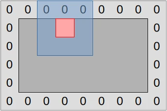
This approach to edge handling has pros and cons:

• Our code logic will be simpler, which seems good as GPU hardware tends to sacrifice some ability to handle fancy code logic in the name of increased number-crunching poser.
• We will need to be more careful with our data layout computations, adding/subtracting 1 to positions and 2 to storage width/height when appropriate. Basically, there is now a difference between working in the space of simulated concentration values (inner dark gray rectangle in diagram above) and the space of actual storage buffers (outer light gray rectangle), and when we switch between the two in our code we need to perform a coordinate transform.
• We may or may not get memory access alignment issues that can reduce our computational performance on some hardware. If we get them, we can resolve them through clever use of extra unused padding floats. But as GPU hardware is known to be more tolerant of unaligned SIMD accesses than CPU hardware, we will not attempt to resolve this issue unless a GPU profiler tells us that we are having it on some particular hardware of interest.

To handle the “careful layout” part of this tradeoff, we will set up a few GLSL utilities that let us share more code between our two compute shaders, so that at least we only need to write the tricky data layout concern once, and can change more easily change the data layout later if needed:

// Data padding control and handling
const uint PADDING_PER_SIDE = 1;
const uint PADDED_UV_WIDTH = UV_WIDTH + 2 * PADDING_PER_SIDE;
//
// Unlike the above constants, these functions will not be zero cost. However
// all their data inputs are either constant across an entire compute
// dispatch's lifetime (data length()) or compilation constants, so the compiler
// should be able to deduplicate multiple calls to them given enough inlining.
uint padded_uv_height() { return Input[0].data.length() / PADDED_UV_WIDTH; }
uint uv_height() { return padded_uv_height() - 2 * PADDING_PER_SIDE; }

// First/last output position that corresponds to an actual data location and
// not a padding value that should always be zero, followed by other useful
// special 2D indices within the simulation domain
const uvec2 DATA_START_POS = uvec2(PADDING_PER_SIDE, PADDING_PER_SIDE);
uvec2 padded_end_pos() {
    return uvec2(PADDED_UV_WIDTH, padded_uv_height());
}
uvec2 data_end_pos() {
    return padded_end_pos() - uvec2(PADDING_PER_SIDE);
}

// Convert a 2D location into a linear buffer index
uint pos_to_index(uvec2 pos) {
    return pos.x + pos.y * PADDED_UV_WIDTH;
}

// Read an (U, V) pair from a particular input location
//
// pos starts at (0, 0) for the upper-left padding value, with (1, 1)
// corresponding to the first actual data value.
vec2 read(uvec2 pos) {
    const uint index = pos_to_index(pos);
    return vec2(
        Input[U].data[index],
        Input[V].data[index]
    );
}

// Write an (U, V) to a particular output location, pos works as in read()
void write(uvec2 pos, vec2 value) {
    const uint index = pos_to_index(pos);
    Output[U].data[index] = value.x;
    Output[V].data[index] = value.y;
}

And that will be it for the code that is shared between our two compute shaders. You can now save all of the above GLSL code, except for the initial #version 460 directive (we’ll get back to this), into a file that at location exercises/src/grayscott/common.comp. And once that is done, we will start writing some actual compute shaders.

Initialization shader

Now that we have some common utilities to interface with our datasets and configure the simulation, let us write out initialization compute shader.

This will mostly be a straightforward GLSL translation of our CPU data initialization code. But because this is GPU code, we need to make a new decision, which is the way GPU work items and workgroups will map onto the work to be done.

We have decided to go with the simple mapping illustrated by the following diagram:

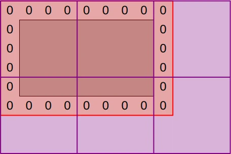
The CPU command buffer that will eventually execute this compute shader will dispatch enough workgroups (purple squares) to cover the full padded simulation dataset (red zone) with one work item per data point. But work item tasks will vary:

• Padding elements (denoted “0”) will be initialized to zero as they should.
• Non-padding elements (inside the zero padding) will be initialized as in the CPU version.
• Out-of bounds work items (outer purple area) will exit early without doing anything.

This general scheme of having work-items at different position perform different kinds of work will reduce execution efficiency a bit on SIMD GPU hardware, however…

• The impact should be minor at the target dataset size of full HD images (1920x1080 concentration values), where edge elements and out-of-bounds work items should only have a small contribution to the overall execution time.
• The initialization compute shader will only execute once per full simulation run, so unless we have reasons to care about the performance of short simulation runs with very few simulation steps, we should not worry about the performance of this shader that much.

All said and done, we can implement the initialization shader using the following GLSL code…

#version 460

#include "common.comp"

// Polyfill for the standard Rust saturating_sub utility
uint saturating_sub(uint x, uint y) {
    if (x >= y) {
        return x - y;
    } else {
        return 0;
    }
}

// Data initialization entry point
void main() {
    // Map work items into 2D padded buffer, discard out-of-bounds work items
    const uvec2 pos = uvec2(gl_GlobalInvocationID.xy);
    if (any(greaterThanEqual(pos, padded_end_pos()))) {
        return;
    }

    // Fill in zero boundary condition at edge of simulation domain
    if (
        any(lessThan(pos, DATA_START_POS))
        || any(greaterThanEqual(pos, data_end_pos()))
    ) {
        write(pos, vec2(0.0));
        return;
    }

    // Otherwise, replicate standard Gray-Scott pattern in central region
    const uvec2 data_pos = pos - DATA_START_POS;
    const uvec2 pattern_start = uvec2(
        7 * UV_WIDTH / 16,
        saturating_sub(7 * uv_height() / 16, 4)
    );
    const uvec2 pattern_end = uvec2(
        8 * UV_WIDTH / 16,
        saturating_sub(8 * uv_height() / 16, 4)
    );
    const bool pattern = all(greaterThanEqual(data_pos, pattern_start))
                         && all(lessThan(data_pos, pattern_end));
    write(pos, vec2(1.0 - float(pattern), float(pattern)));
}

…which should be saved at location exercises/src/grayscott/init.comp.

As is customary in this course, we will point out a few things about the above code:

• Like C, GLSL supports #include preprocessor directives that can be used in order to achieve a limited from of software modularity. Here we are using it to make our two compute shaders share a common CPU-GPU interface and a few common utility constants/functions.
• …but for reasons that are not fully clear to the course’s author (dubious GLSL design decision or shaderc compiler bug?), #version directives cannot be extracted into a common GLSL source file and must be present in the source code of each individual compute shader.
• GLSL provides built-in vector and matrix types, which we use here in an attempt to make our 2D computations a little clearer. Use of these types may sometimes be required for performance (especially when small data types like 8-bit integers and half-precision floating point numbers get involved), but here we only use them for expressivity and concision.

Simulation shader

In the initialization shader that we have just covered, we needed to initialize the entire GPU dataset, padding edges included. And the most obvious way to do this was to map each GPU work item into one position of the full GPU dataset, padding zeroes included.

When it comes to the subsequent Gray-Scott reaction simulation, however, the mapping between work items and data that we should use is less immediately obvious. The two simplest approaches would be to use one work item per input data point (which would include padding, as in our initialization algorithm) or one work item per updated output U/V value (excluding padding). But these approaches entail different tradeoffs:

• Using one work item per input data point allows us to expose a bit more concurrent work to the GPU (one extra work item per padding element), but as mentioned earlier the influence of such edges should be negligible when computing a larger image of size 1920x1080.
• Using one work item per output data point means that each GPU work item can load all of its data inputs without cooperating with other work items, and is the only writer of its data output. But this comes at the expense of each input value being redundantly loaded ≤8 more times by the Laplacian computations associated with all output data points at neighboring 2D positions. This may or may not be automatically handled by the GPU’s cache hierarchy.
• In contrast, with one work item per input data point, we will perfom no redundant data loading work, but will need to synchronize work items with each other in order to perform the Laplacian computation, because a Laplacian computation’s inputs now come from multiple work items. Synchronization comes at the expense of extra code complexity, and also adds some overhead that may negate the benefits of avoiding redundant memory loads.

Since there is no obviously better approach here, it is best to try both and compare their performance. Therefore, in the initial version of our Gray-Scott GPU implementation we will start with the simplest code of using one work item per output data point, which is illustrated below. And later on, after we get a basic simulation working, we will discuss optimizations that reduce the costs of redundant Laplacian input loading or eliminate such redundant loading entirely.

The following diagram summarizes the resulting execution and data access strategy:

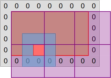
CPU command buffers that will execute the simulation compute shader will dispatch enough workgroups (purple squares) to cover the central region of the simulation dataset (red rectangle) with one work item per output data point. On the GPU side, work items that map into a padding or out-of-bounds location (purple area) will be discarded by exiting main() early.

Each remaining work item will then proceed to compute the updated (U, V) pair associated with its output location, as illustrated by the concentric blue and red squares:

• The work-item will load the current (U, V) value associated with its assigned output location (red square) and all neighboring input values (blue square) from the input buffers.
• It will then perform computations based one these inputs that will eventually produce an updated (U, V) value, which will be written down to the matching location of the output buffers.

This results in the following GLSL code…

#version 460

#include "common.comp"

// Simulation step entry point
void main() {
    // Map work items into 2D central region, discard out-of-bounds work items
    const uvec2 pos = uvec2(gl_GlobalInvocationID.xy) + DATA_START_POS;
    if (any(greaterThanEqual(pos, data_end_pos()))) {
        return;
    }

    // Load central value
    const vec2 uv = read(pos);

    // Compute the diffusion gradient for U and V
    const uvec2 topleft = pos - uvec2(1);
    const mat3 weights = stencil_weights();
    vec2 full_uv = vec2(0.0);
    for (int y = 0; y < 3; ++y) {
        for (int x = 0; x < 3; ++x) {
            const vec2 stencil_uv = read(topleft + uvec2(x, y));
            full_uv += weights[x][y] * (stencil_uv - uv);
        }
    }

    // Deduce the change in U and V concentration
    const float u = uv.x;
    const float v = uv.y;
    const float uv_square = u * v * v;
    const vec2 delta_uv = diffusion_rate() * full_uv + vec2(
        FEED_RATE * (1.0 - u) - uv_square,
        uv_square - (FEED_RATE + KILL_RATE) * v
    );
    write(pos, uv + delta_uv * DELTA_T);
}

…which sould be saved at location exercises/src/grayscott/step.comp.

SPIR-V interface

Now that the GLSL is taken care of, it is time to work on the Rust side. Inside of exercises/src/grayscott/pipeline.rs, let’s ask vulkano to build the SPIR-V shader modules and create some Rust-side constants mirroring the GLSL specialization constants as we did before…

/// Shader modules used for the compute pipelines
mod shader {
    vulkano_shaders::shader! {
        shaders: {
            init: {
                ty: "compute",
                path: "src/grayscott/init.comp"
            },
            step: {
                ty: "compute",
                path: "src/grayscott/step.comp"
            },
        }
    }
}

/// Descriptor set that is used to bind input and output buffers to the shader
pub const INOUT_SET: u32 = 0;

// Descriptor array bindings within INOUT_SET, in (U, V) order
pub const IN: u32 = 0;
pub const OUT: u32 = 1;

// === Specialization constants ===
//
// Workgroup size
const WORKGROUP_SIZE_X: u32 = 0;
const WORKGROUP_SIZE_Y: u32 = 1;
//
/// Concentration table width
const UV_WIDTH: u32 = 2;
//
// Scalar simulation parameters
const FEED_RATE: u32 = 3;
const KILL_RATE: u32 = 4;
const DELTA_T: u32 = 5;
//
/// Start of 3x3 Laplacian stencil
const STENCIL_WEIGHT_START: u32 = 6;
//
// Diffusion rates of U and V
const DIFFUSION_RATE_U: u32 = 15;
const DIFFUSION_RATE_V: u32 = 16;

…which will save us from the pain of figuring out magic numbers in the code later on.

Notice that in the code above, we use a variation of the default vulkano_shaders syntax, which allows us to build multiple shaders at once. This makes some things more convenient, for example auto-generated Rust structs will be deduplicated, and it is possible to set some vulkano_shaders options once for all the shaders that we are compiling.

Specialization

As in the CPU version, our GPU compute pipeline will be tunable via a set of CLI options:

• We will retain the UpdateOptions used to tune the CPU simulation, which also apply here.
• We will supplement these with a pair of options that control the GPU workgroup size, by creating a new PipelineOptions struct that encompasses everything.
• We will modify the global RunnerOptions to feature PipelineOptions instead of UpdateOptions, so that all CLI options are available in the final program.

Overall, this results in the following code changes:

// Add pipeline options to pipeline.rs...

use super::options::UpdateOptions;
use clap::Args;
use std::num::NonZeroU32;

/// CLI parameters that guide pipeline creation
#[derive(Debug, Args)]
pub struct PipelineOptions {
    /// Number of rows in a workgroup
    #[arg(short = 'R', long, default_value = "8")]
    pub workgroup_rows: NonZeroU32,

    /// Number of columns in a workgroup
    #[arg(short = 'C', long, default_value = "8")]
    pub workgroup_cols: NonZeroU32,

    /// Options controlling simulation updates
    #[command(flatten)]
    pub update: UpdateOptions,
}

// ...then integrate these options into the RunnerOptions of options.rs

use super::pipeline::PipelineOptions;

#[derive(Debug, Parser)]
#[command(version)]
pub struct RunnerOptions {
    // [ ... taking the place of UpdateOptions ... ]

    /// Options controlling the simulation pipeline
    #[command(flatten)]
    pub pipeline: PipelineOptions,
}

Once this is done, the RunnerOptions will contain all the information we need to specialize our GPU shader modules, which we will do using the following function:

// Back to pipeline.rs

use super::options::{self, RunnerOptions, STENCIL_WEIGHTS};
use crate::Result;
use std::sync::Arc;
use vulkano::{
    shader::{ShaderModule, SpecializationConstant, SpecializedShaderModule},
};

/// Set up a specialized shader module with a certain workgroup size
fn setup_shader_module(
    options: &RunnerOptions,
    module: Arc<ShaderModule>,
) -> Result<Arc<SpecializedShaderModule>> {
    // Set specialization constants. We'll be less careful this time because
    // there are so many of them in this kernel
    let mut constants = module.specialization_constants().clone();
    assert_eq!(
        constants.len(),
        17,
        "unexpected amount of specialization constants"
    );
    use SpecializationConstant::{F32, U32};
    //
    let pipeline = &options.pipeline;
    *constants.get_mut(&WORKGROUP_SIZE_X).unwrap() = U32(pipeline.workgroup_cols.get());
    *constants.get_mut(&WORKGROUP_SIZE_Y).unwrap() = U32(pipeline.workgroup_rows.get());
    //
    *constants.get_mut(&UV_WIDTH).unwrap() = U32(options.num_cols as _);
    //
    let update = &pipeline.update;
    *constants.get_mut(&FEED_RATE).unwrap() = F32(update.feedrate);
    *constants.get_mut(&KILL_RATE).unwrap() = F32(update.killrate);
    *constants.get_mut(&DELTA_T).unwrap() = F32(update.deltat);
    //
    for (offset, weight) in STENCIL_WEIGHTS.into_iter().flatten().enumerate() {
        *constants
            .get_mut(&(STENCIL_WEIGHT_START + offset as u32))
            .unwrap() = F32(weight);
    }
    //
    *constants.get_mut(&DIFFUSION_RATE_U).unwrap() = F32(options::DIFFUSION_RATE_U);
    *constants.get_mut(&DIFFUSION_RATE_V).unwrap() = F32(options::DIFFUSION_RATE_V);

    // Specialize the shader module accordingly
    Ok(module.specialize(constants)?)
}

Careful readers of the square code will notice that the API design here is a little different from what we had before. We used to load the shader module inside of setup_shader_module(), whereas now we ask the caller to load the shader module and pass it down.

The reason for this change is that now we have two different compute shaders to take care of (one initialization shader and one simulation shader), and we want to set the same specialization constant work for both of them. The aforementioned API design change lets us do that.

Multiple shaders, single layout

As in the previous square example, our two compute shaders will each have a single entry point. Which means that we can reuse the previous setup_compute_stage() function:

/// Set up a compute stage from a previously specialized shader module
fn setup_compute_stage(module: Arc<SpecializedShaderModule>) -> PipelineShaderStageCreateInfo {
    let entry_point = module
        .single_entry_point()
        .expect("a compute shader module should have a single entry point");
    PipelineShaderStageCreateInfo::new(entry_point)
}

However, if we proceed to do everything else as in the square example, we will end up with two compute pipeline layouts, which means that we will need two versions of each resource descriptor set we create, one per compute pipeline. This sounds a little ugly and wasteful, so we would like to get our two compute pipelines to share a common pipeline layout.

Vulkan supports this by allowing a pipeline’s layout to describe a superset of the resources that the pipeline actually uses. If we consider our current GPU code in the eyes of this rule, this means that a pipeline layout for the step compute shader can also be used with the init compute shader, because the set of resources that init uses (Output storage block) is a subset of the set of resources that step uses (Input and Output storage blocks).

But from a software maintainability perspective, we would rather not hardcode the assumption that the step pipeline will forever use a strict superset of the resources used by all other GPU pipelines, as we might later want to e.g. adjust the definition of init in a manner that uses resources that step doesn’t need. Thankfully we do not have to go there.

The PipelineDescriptorSetLayoutCreateInfo convenience helper from vulkano that we have used earlier is not limited to operating on a single GPU entry point. Its constructor actually accepts an iterable set of PipelineStageCreateInfo, and if you provide multiple ones it will attempt to produce a pipeline layout that is compatible with all of the underlying entry points by computing the union of their layout requirements.

Obviously, this layout requirements union computation will only work if the the entry points do not have incompatible layout requirement (e.g. one declares that set 0, binding 0 maps into a buffer while the other declares that it is an image). But there is not risk of this happening to us here as both compute shaders share the same CPU-GPU interface specification from common.comp. So we can safely use this vulkano functionality as follows:

use vulkano::{
    descriptor_set::layout::DescriptorType,
    pipeline::layout::{PipelineDescriptorSetLayoutCreateInfo, PipelineLayout},
};

/// Set up the compute pipeline layout
fn setup_pipeline_layout<const N: usize>(
    device: Arc<Device>,
    stages: [&PipelineShaderStageCreateInfo; N],
) -> Result<Arc<PipelineLayout>> {
    // Auto-generate a sensible pipeline layout config
    let layout_info = PipelineDescriptorSetLayoutCreateInfo::from_stages(stages);

    // Check that the pipeline layout meets our expectation
    //
    // Otherwise, the GLSL interface was likely changed without updating the
    // corresponding CPU code, and we just avoided rather unpleasant debugging.
    assert_eq!(
        layout_info.set_layouts.len(),
        1,
        "this program should only use a single descriptor set"
    );
    let set_info = &layout_info.set_layouts[INOUT_SET as usize];
    assert_eq!(
        set_info.bindings.len(),
        2,
        "the only descriptor set should contain two bindings"
    );
    let input_info = set_info
        .bindings
        .get(&IN)
        .expect("an input data binding should be present");
    assert_eq!(
        input_info.descriptor_type,
        DescriptorType::StorageBuffer,
        "the input data binding should be a storage buffer binding"
    );
    assert_eq!(
        input_info.descriptor_count, 2,
        "the input data binding should contain U and V data buffer descriptors"
    );
    let output_info = set_info
        .bindings
        .get(&OUT)
        .expect("an output data binding should be present");
    assert_eq!(
        output_info.descriptor_type,
        DescriptorType::StorageBuffer,
        "the output data binding should be a storage buffer binding"
    );
    assert_eq!(
        output_info.descriptor_count, 2,
        "the output data binding should contain U and V data buffer descriptors"
    );
    assert!(
        layout_info.push_constant_ranges.is_empty(),
        "this program shouldn't be using push constants"
    );

    // Finish building the pipeline layout
    let layout_info = layout_info.into_pipeline_layout_create_info(device.clone())?;
    let layout = PipelineLayout::new(device, layout_info)?;
    Ok(layout)
}

Exercise

We now have all the building blocks that we need in order to build Vulkan compute pipelines for our data-initialization and simulation shaders, with a shared layout that will later allow us to have common descriptor sets for all pipelines. Time to put it all together into a single struct:

use crate::context::Context;
use vulkano::pipeline::compute::ComputePipeline;

/// Initialization and simulation pipelines with common layout information
#[derive(Clone)]
pub struct Pipelines {
    /// Compute pipeline used to initialize the concentration tables
    pub init: Arc<ComputePipeline>,

    /// Compute pipeline used to perform a simulation step
    pub step: Arc<ComputePipeline>,

    /// Pipeline layout shared by `init` and `step`
    pub layout: Arc<PipelineLayout>,
}
//
impl Pipelines {
    /// Set up all the compute pipelines
    pub fn new(options: &RunnerOptions, context: &Context) -> Result<Self> {
        // TODO: Implement all these functions
    }
}

Your goal for this chapter’s exercise will be to take inspiration from the equivalent struct in the number-squaring pipeline that we studied earlier, and use this inspiration implement the new() constructor for our new set of compute pipelines.

Then you will create (for now unused) Pipelines at the start of the run_simulation() body (in exercises/src/grayscott/mod.rs). And after that you will make sure that debug builds of said binary executes without any error or unexpected warning from the Vulkan validation layers.

Finally, if you are a more experienced Rust developer and want to practice your generics a bit, you may also try deduplicating the logic associated with the init and step entry points inside of the Pipelines::new() constructor.

1. Being aware of this major shortcoming of traditional CPU programming, GPUs also support multi-dimensional image resources backed by specialized texturing hardware, which should provide better performance than 1D buffer indexing code that emulates 2D indexing. So the author of this course tried to use these… and experienced great disappointment. Ask for the full story. ↩

Data & I/O

As before, after setting up our GPU compute pipelines, we will want to set up some data buffers that we can bind to those pipelines.

This process will be quite a bit simpler than before because we will not repeat the introduction to Vulkan memory management and will be using GPU-side initialization. So we will use the resulting savings in character budget to…

• Show what it takes to integrate GPU data into our existing CPU simulation skeleton.
• Follow the suggestion made in the number-squaring chapter to avoid having a single build_command_buffer() god-function that does all command buffer building.
• Adjust our HDF5 I/O logic so that we do not need to download U concentration from the GPU.

GPU dataset

New code organization

The point of Vulkan descriptor sets is to allow your application to use as few of them as possible in order to reduce resource binding overhead. In the context of our Gray-Scott simulation, the lowest we can easily¹ achieve is to have two descriptor sets.

• One that uses two buffers (let’s call them U1 and V1) as inputs and two other buffers (let’s call them U2 and V2) as outputs.
• Another that uses the same buffers, but flips the roles of input and output buffers. Using the above notation, U2 and U2 become the inputs, while U1 and U1 become the outputs.

Given this descriptor set usage scheme, our command buffers will alternatively bind these two descriptor sets, executing the simulation compute pipeline after each descriptor set binding call, and this will roughly replicate the double buffering pattern that we used on the CPU.

To get there, however, we will need to redesign our inner data abstractions a bit with respect to what we used to have on the CPU side. Indeed, back in the CPU course, we used to have the following separation of concerns in our code:

• One struct called UV would represent a pair of tables of identical size and related contents, one representing the chemical concentration of species U and one representing the chemical concentration of species V.
• Another struct called Concentrations would represent a pair of UV structs and implement the double buffering logic for alternatively using one of these UV structs to store inputs, and the other to store outputs.

But now that we have descriptor sets that combine inputs and outputs, this program decomposition scheme doesn’t work anymore. Which is why we will have to switch to a different scheme:

• One struct called InOut will contain and manage all vulkano objects associated to one (U, V) input pair and one (U, V) output pair.
• struct Concentrations will remain around, but be repurposed to manipulate pairs of InOut rather than pairs of UV. And users of its update() function will now only be exposed to a single DescriptorSet, instead of being exposed to a pair of UVs as in the CPU code.

Introducing InOut

Our new InOut data structure is going to look like this:

use std::sync::Arc;
use vulkano::{buffer::subbuffer::Subbuffer, descriptor_set::DescriptorSet};

/// Set of GPU inputs and outputs
struct InOut {
    /// Descriptor set used by GPU compute pipelines
    descriptor_set: Arc<DescriptorSet>,

    /// Input buffer for the V species, used during GPU-to-CPU data transfers
    input_v: Subbuffer<[Float]>,
}

As the comments point out, we are going to keep both a full input/output descriptor set and a V input buffer around, because they are useful for different tasks:

• Compute pipeline execution commands operate over descriptor sets
• Buffer-to-buffer data transfer commands operate over the underlying Subbuffer objects
• Because descriptor sets are a very general-purpose abstraction, going from a descriptor set to the underlying buffer objects is a rather cumbersome process.
• And because Subbuffer is jute a reference-counted pointer, it does not cost much performance to skip that cumbersome process by keeping around a V buffer reference.

Notice that we do not keep around the Subbuffer associated with the U species’ concentration, because we do not actually need it. We will get back to this.

For now, let us look at how an InOut is constructed:

use super::{
    options::RunnerOptions,
    pipeline::{IN, INOUT_SET, OUT},
};
use crate::{context::Context, Result};
use vulkano::{
    buffer::{Buffer, BufferCreateInfo, BufferUsage},
    descriptor_set::WriteDescriptorSet,
    memory::allocator::AllocationCreateInfo,
    pipeline::layout::PipelineLayout,
    DeviceSize,
};

/// Number of padding elements per side of the simulation domain
const PADDING_PER_SIDE: usize = 1;

/// Compute the padded version of a simulation dataset dimension (rows/cols)
fn padded(dimension: usize) -> usize {
    dimension + 2 * PADDING_PER_SIDE
}

impl InOut {
    /// Allocate a set of 4 buffers that can be used to store either U and V
    /// species concentrations, and can serve as inputs or outputs
    fn allocate_buffers(
        options: &RunnerOptions,
        context: &Context,
    ) -> Result<[Subbuffer<[Float]>; 4]> {
        use BufferUsage as BU;
        let padded_rows = padded(options.num_rows);
        let padded_cols = padded(options.num_cols);
        let new_buffer = || {
            Buffer::new_slice(
                context.mem_allocator.clone(),
                BufferCreateInfo {
                    usage: BU::STORAGE_BUFFER | BU::TRANSFER_DST | BU::TRANSFER_SRC,
                    ..Default::default()
                },
                AllocationCreateInfo::default(),
                (padded_rows * padded_cols) as DeviceSize,
            )
        };
        Ok([new_buffer()?, new_buffer()?, new_buffer()?, new_buffer()?])
    }

    /// Set up an `InOut` configuration by assigning roles to the 4 buffers that
    /// [`allocate_buffers()`](Self::allocate_buffers) previously allocated
    fn new(
        context: &Context,
        layout: &PipelineLayout,
        input_u: Subbuffer<[Float]>,
        input_v: Subbuffer<[Float]>,
        output_u: Subbuffer<[Float]>,
        output_v: Subbuffer<[Float]>,
    ) -> Result<Self> {
        // Determine how the descriptor set will bind to the compute pipeline
        let set_layout = layout.set_layouts()[INOUT_SET as usize].clone();

        // Configure what resources will attach to the various bindings
        // that the descriptor set is composed of
        let descriptor_writes = [
            WriteDescriptorSet::buffer_array(IN, 0, [input_u.clone(), input_v.clone()]),
            WriteDescriptorSet::buffer_array(OUT, 0, [output_u.clone(), output_v.clone()]),
        ];

        // Set up the descriptor set according to the above configuration
        let descriptor_set = DescriptorSet::new(
            context.desc_allocator.clone(),
            set_layout,
            descriptor_writes,
            [],
        )?;

        // Also keep track of the V input buffer, and we're done
        Ok(Self {
            descriptor_set,
            input_v,
        })
    }
}

The general idea here is that because our two InOuts will refer to the same buffers, we cannot allocate the buffers internally inside of the InOut::new() constructor. Instead we will need to allocate buffers inside of the code from Concentrations that builds InOuts, then use the same buffers twice in a different order to build the two different InOuts.

It is not so nice from an abstraction design point of view that the caller needs to know about such a thing as the right order in which buffers should be passed. But sadly this cannot be cleanly fixed at the InOut layer, so we will fix it at the Concentrations layer instead.

Updating Concentrations

In the CPU simulation, the Concentrations struct used to…

• Contain a pair of UV values and a boolean that clarified their input/output role
• Offload most initialization work to the lower UV layer
• Expose an update() method whose user callback received both an immutable input (&UV) and a mutable output (&mut UV)

For the GPU simulation, as discussed earlier, we will switch to a different architecture:

• Concentrations will now contain InOuts instead of UVs
• InOut initialization will now be handled by the Concentrations layer, as it is the one that has easy access to the output buffers of each InOut
• Initialization will now be asynchronous, as it entails some Vulkan commands that must be enqueued inside of a command buffer
• The update() method will only receive a single DescriptorSet, as this contains all info needed to read inputs and write outputs

The switch to InOut is straightforward enough, and probably not worth discussing…

/// Double-buffered chemical species concentration storage
pub struct Concentrations {
    /// Compute pipeline input/output configurations
    ///
    /// If we denote `(U1, V1, U2, V2)` the underlying storage buffers...
    /// - The first "forward" configuration uses `(U1, V1)` as inputs and
    ///   `(U2, V2)` as outputs.
    /// - The second "reverse" configuration uses `(U2, V2)` as inputs and
    ///   `(U1, V1)` as outputs.
    ///
    /// By alternating between these two configurations, we can take as many
    /// simulation steps as we need to, always using the output of the
    /// simulation step N as the input of simulation step N+1.
    inout_sets: [InOut; 2],

    /// Truth that the second "revese" input/output configuration is active
    reversed: bool,
}

…however the constructor change will be quite a bit more substantial:

use super::{
    pipeline::Pipelines,
    CommandBufferBuilder,
};
use std::num::NonZeroU32;
use vulkano::pipeline::PipelineBindPoint;

impl Concentrations {
    /// Set up GPU data storage and schedule GPU buffer initialization
    ///
    /// GPU buffers will only be initialized after the command buffer associated
    /// with `cmdbuild` has been built and submitted for execution. Any work
    /// that depends on their initial value must be scheduled afterwards.
    pub fn create_and_schedule_init(
        options: &RunnerOptions,
        context: &Context,
        pipelines: &Pipelines,
        cmdbuild: &mut CommandBufferBuilder,
    ) -> Result<Self> {
        // Allocate all GPU storage buffers used by the simulation
        let [u1, v1, u2, v2] = InOut::allocate_buffers(options, context)?;

        // Set up input/output configurations
        let inout1 = InOut::new(
            context,
            &pipelines.layout,
            u1.clone(),
            v1.clone(),
            u2.clone(),
            v2.clone(),
        )?;
        let inout2 = InOut::new(context, &pipelines.layout, u2.clone(), v2.clone(), u1, v1)?;

        // Schedule initialization using the second descriptor set. The output
        // buffers of this descriptor set are the input buffers of the first
        // descriptor set, which will be used first.
        cmdbuild.bind_pipeline_compute(pipelines.init.clone())?;
        cmdbuild.bind_descriptor_sets(
            PipelineBindPoint::Compute,
            pipelines.layout.clone(),
            INOUT_SET,
            inout2.descriptor_set.clone(),
        )?;
        let num_workgroups = |domain_size: usize, workgroup_size: NonZeroU32| {
            padded(domain_size).div_ceil(workgroup_size.get() as usize) as u32
        };
        let padded_workgroups = [
            num_workgroups(options.num_cols, options.pipeline.workgroup_cols),
            num_workgroups(options.num_rows, options.pipeline.workgroup_rows),
            1,
        ];
        // SAFETY: GPU shader has been checked for absence of undefined behavior
        //         given a correct execution configuration, and this is one
        unsafe {
            cmdbuild.dispatch(padded_workgroups)?;
        }

        // Schedule zero-initialization of the edges of the first output.
        //
        // Only the edges need to be initialized. The values at the center of
        // the dataset do not matter, as these buffers will serve as simulation
        // outputs at least once (which will initialize their central values)
        // before they serve as a simulation input.
        //
        // Here we initialize the entire buffer to zero, as the Vulkan
        // implementation is likely to special-case this buffer-zeroing
        // operation with a high-performance implementation.
        cmdbuild.fill_buffer(u2.reinterpret(), 0)?;
        cmdbuild.fill_buffer(v2.reinterpret(), 0)?;

        // Once the command buffer is executed, everything will be ready
        Ok(Self {
            inout_sets: [inout1, inout2],
            reversed: false,
        })
    }

    // [ ... more methods coming up ... ]
}

As you can see, it is now the Concentrations constructor that is responsible for allocating storage for the underlying InOut structs and assigning input and output roles to it.

The initialization process also becomes a bit more complex:

• The true simulation input is initialized using the init compute pipeline introduced earlier.
• The other set of (U, V) buffers must now be initialized because we now use a zero-padding scheme to handle simulation domain edges. We do this by filling these buffers with zeroes, which is overkill but likely to be optimized in hardware.
• Both of these operations are asynchronous Vulkan commands, so usage of the Concentrations is now a bit more complex as it now builds a command buffer that must be submitted to the GPU and executed. We acknowledge this by switching from the standard new() constructor naming to a more complex create_and_schedule_init() name that highlights what the user of this function needs to do.

When it comes to accessors, shape() will be dropped as it cannot be easily provided by our 1D GPU storage without keeping otherwise unnecessary metadata around. But the current() accessor will trivially be migrated to the new logic. And for reasons that will become clear later on, it can also become a private implementation detail of the underlying data module.

impl Concentrations {
    // [ ... ]

    /// Current input/output configuration
    fn current_inout(&self) -> &InOut {
        &self.inout_sets[self.reversed as usize]
    }

    // [ ... ]
}

On its side, the update() operation will be easily migrated to the new logic discussed above as well, as it is largely a simplification with respect to its former implementation:

impl Concentrations {
    // [ ... ]


    /// Run a simulation step
    ///
    /// The `step` callback will be provided with the descriptor set that should
    /// be used for the next simulation step. If you need to carry out multiple
    /// simulation steps, you should call `update()` once per simulation step.
    pub fn update(&mut self, step: impl FnOnce(Arc<DescriptorSet>) -> Result<()>) -> Result<()> {
        step(self.current_inout().descriptor_set.clone())?;
        self.reversed = !self.reversed;
        Ok(())
    }
}

There is just one new thing that we will need for GPU computing, which is the ability to report errors from GPU programs. This is handled by making the inner step callback return a Result<()>.

Output retrieval & storage

While InOut and Concentrations are enough for the purpose of setting up the simulation and running simulation steps, we are going to need one more thing for the purpose of retrieving GPU output on the CPU side. Namely a Vulkan buffer that the CPU can access.

We could adapt the old UV struct for this purpose, but if you pay attention to how the simulation output is actually used, you will notice that the io module only writes the V species’ concentration to the HDF5 file. And while passing an entire UV struct to this module anyway was fine when direct data access was possible, it is becoming wasteful if we now need to perform an expensive GPU-to-CPU transfer of the full (U, V) dataset only to use the V part exclusively later on.

Therefore, our new VBuffer abstraction will focus on retrieval of the V species’ concentration only.

The construction code is quite similar to the one seen before in InOut::allocate_buffers() (and in fact could be deduplicated with respect to it in a more production-grade codebase). The only thing that changed is that the BufferUsage and AllocationCreateInfo have been adjusted to make this buffer fit for the purpose of downloading data to the CPU:

/// CPU-accessible storage buffer used to download the V species' concentration
pub struct VBuffer {
    /// Buffer in which GPU data will be downloaded
    buffer: Subbuffer<[Float]>,

    /// Number of columns in the 2D concentration table, including zero padding
    padded_cols: usize,
}
//
impl VBuffer {
    /// Set up a `VBuffer`
    pub fn new(options: &RunnerOptions, context: &Context) -> Result<Self> {
        use vulkano::memory::allocator::MemoryTypeFilter as MTFilter;
        let padded_rows = padded(options.num_rows);
        let padded_cols = padded(options.num_cols);
        let buffer = Buffer::new_slice(
            context.mem_allocator.clone(),
            BufferCreateInfo {
                usage: BufferUsage::TRANSFER_DST,
                ..Default::default()
            },
            AllocationCreateInfo {
                memory_type_filter: MTFilter::PREFER_HOST | MTFilter::HOST_RANDOM_ACCESS,
                ..Default::default()
            },
            (padded_rows * padded_cols) as DeviceSize,
        )?;
        Ok(Self {
            buffer,
            padded_cols,
        })
    }

    // [ ... more methods coming up ... ]
}

After that, we can add a method to schedule a GPU-to-CPU data transfer…

use vulkano::command_buffer::CopyBufferInfo;

impl VBuffer {
    // [ ... ]

    /// Schedule a download of some [`Concentrations`]' current V input into
    /// the internal CPU-accessible buffer of this `VBuffer`
    ///
    /// The GPU-to-CPU download will only begin after the command buffer
    /// associated with `cmdbuild` has been built and submitted to the GPU for
    /// execution. You must wait for the associated GPU work to complete before
    /// processing the output with the [`process()`](Self::process) method.
    pub fn schedule_download(
        &mut self,
        source: &Concentrations,
        cmdbuild: &mut CommandBufferBuilder,
    ) -> Result<()> {
        cmdbuild.copy_buffer(CopyBufferInfo::buffers(
            source.current_inout().input_v.clone(),
            self.buffer.clone(),
        ))?;
        Ok(())
    }

    // [ ... ]
}

…and there is just one last piece to take care of, which is to provide a way to access the inner data after the download is complete. Which will require a bit more work than you may expect.

To set the stage, let’s point out that we are trying to set up some communication between two Rust libraries with the following API design.

• To avoid data races between the CPU and the GPU, vulkano enforces an RAII design where accesses to a Subbuffer must go through the Subbuffer::read() method. This method returns a BufferReadGuard that borrows from the underlying Subbuffer and lets vulkano know at destruction time that it is not being accessed by the CPU anymore. Under the hood, locks and checks are then used to achieve thread safety.
• We start from this BufferReadGuard, which borrows memory from the underlying Subbuffer storage like a standard Rust slice of type &[Float] could borrow from a Vec<Float>. And we want to add 2D layout information in order to turn it into an ndarray::ArrayView2<Float>, which is what the HDF5 binding that we are using ultimately expects.

Now, because the VBuffer type that we are building is logically a 2D array, it would be good API design from our side to refrain from exposing the underlying 1D vulkano dataset in the VBuffer API and instead only provide users with the ArrayView2 that they need for HDF5 I/O and other operations. While we are at it, we would also rather not expose the zero padding elements to the user, as they won’t be part of the final HDF5 file and are arguably an implementation detail of our current Gray-Scott simulation implementation.

We can get all of those good things, as it turns out, but the simplest way for us to get there² will be a somewhat weird callback-based interface:

use ndarray::prelude::*;

impl VBuffer {
    // [ ... ]

    /// Process the latest download of the V species' concentrations
    ///
    /// Before calling this method, you will want to [schedule a
    /// download](Self::schedule_download), submit the resulting command buffer,
    /// and await its completion.
    ///
    /// The provided V species concentration table will only contain active
    /// elements, excluding zero-padding elements on the edge.
    pub fn process(&self, callback: impl FnOnce(ArrayView2<Float>) -> Result<()>) -> Result<()> {
        // Access the underlying dataset as a 1D slice
        let read_guard = self.buffer.read()?;

        // Create an ArrayView2 that covers the whole data, padding included
        let padded_cols = self.padded_cols;
        let padded_elements = read_guard.len();
        assert_eq!(padded_elements % padded_cols, 0);
        let padded_rows = padded_elements / padded_cols;
        let padded_view = ArrayView::from_shape([padded_rows, padded_cols], &read_guard)?;

        // Extract the central region of padded_view, excluding padding
        let data_view = padded_view.slice(s!(
            PADDING_PER_SIDE..(padded_rows - PADDING_PER_SIDE),
            PADDING_PER_SIDE..(padded_cols - PADDING_PER_SIDE),
        ));

        // We are now ready to run the user callback
        callback(data_view)
    }
}

The general idea here is that a user who wants to read the contents of the buffer will pass us a function (typically a lambda) that takes the current contents of the buffer (as an un-padded ArrayView2) and returns a Result<()> that tells if the operation is successful.

On our side, we will then do everything needed to set up the two-dimensional array view, pass it to the user-specified callback function, and return the result.

HDF5 I/O refactor

As mentioned earlier, one last thing that should change with respect to our former CPU code is that we want our HDF5 I/O module to be clearer about what it wants.

Indeed, at present time, HDF5Writer::write() demands a full set of (U, V) data of which it only uses the V concentration data. This was fine from a CPU programming perspective where we don’t pay for exposing unused data access opportunities. But from a GPU programming perspective it means downloading U concentration data that the HDF5 I/O module is not going to use.

We will fix this by making the HDF5Writer more explicit about what it wants, and having it take the V species concentration only instead.

// In exercises/src/grayscott/io.rs

use ndarray::ArrayView2;

impl HDF5Writer {
    // [ ... ]

    /// Write a new V species concentration table to the file
    pub fn write(&mut self, v: ArrayView2<Float>) -> hdf5::Result<()> {
        // FIXME: Workaround for an HDF5 binding limitation
        let v = v.to_owned();
        self.dataset.write_slice(&v, (self.position, .., ..))?;
        self.position += 1;
        Ok(())
    }

    // [ ... ]
}

Notice the FIXME above. Apparently, the Rust HDF5 binding we are using does not yet handle ArrayView2s whose rows are not contiguous in memory, which means that we must create a contiguous copy of v before it accepts to write it to a file.

From the author’s understanding of the HDF5 C API, it can handle this, and this is a Rust binding limitation that should be fixed. But until a fix happens, making an owned contiguous copy should be a reasonably efficient workaround, as for typical storage devices in-RAM copies are much faster than writing data to the target storage device.

As an alternative, we could also modify our GPU-to-CPU copy logic so that it does not copy the padding zero elements, saving a bit of CPU-GPU interconnect bandwidth along the way. However this will require us to stop using standard Vulkan copy commands and use custom shaders for this purpose instead, which may in turn cause two issues:

• Performance may be worse, because the standard Vulkan copy command should have been well-optimized by the GPU vendor. Our shader would need to be optimized similarly for all GPU devices on which we want to perform well, which is a lot of work.
• We will very likely lose the ability to overlap GPU-to-CPU copies with computations, which we are not using yet but may want to use later as an optimization.

As always, tradeoffs are the name of the game in engineering… but as you will see later, this particular tradeoff is going to disappear once we introduce other optimizations anyway.

Exercise

In the data module of the Gray-Scott reaction simulation (exercises/src/grayscott/data.rs), replace the UV and Concentrations structs with the InOut, Concentrations and VBuffer types introduced in this chapter.

After that is done, proceed to modify the io module of the simulation so that it works with borrowed V concentration data only, as discussed above.

You will find that the simulation does not compile at this point. This is expected because the run_simulation() and update() function of the simulation library have not been updated yet, and the CommandBufferBuilder type alias has not been defined yet either. We will fix that in the next chapter, for now just make sure that there is no compilation error originating from a mistake in data.rs or io.rs.

1. Without losing the benefits of GLSL’s readonly and writeonly qualifiers and introducing new Vulkan concepts like push constants, that is. ↩

2. It is possible to write a callback-free read() method that returns an object that behaves like an ArrayView2, but implementing it efficiently (without recreating the ArrayView2 on every access) involves building a type that is self-referential in the eyes of the Rust’s compiler lifetime analysis. Which means that some dirty unsafe tricks will be required. ↩

Integration

After a long journey, we are once again reaching the last mile where we almost have a complete Gray-Scott reaction simulation. In this chapter, we will proceed to walk this last mile and get everything working again, on GPU this time.

Command buffer building

As we go through the optimization chapters, we will want to build command buffers for submitting work to the GPU in a growing number of places. Because our needs are rather simple, we will always build them in the same way, which is worth extracting into a utility function and type alias:

use crate::{context::Context, Result};
use vulkano::command_buffer::{
    AutoCommandBufferBuilder, CommandBufferUsage, PrimaryAutoCommandBuffer
};

/// Convenience type alias for primary command buffer builders
type CommandBufferBuilder = AutoCommandBufferBuilder<PrimaryAutoCommandBuffer>;

/// Set up a new command buffer builder
fn command_buffer_builder(context: &Context) -> Result<CommandBufferBuilder> {
    let cmdbuild = CommandBufferBuilder::primary(
        context.comm_allocator.clone(),
        context.queue.queue_family_index(),
        CommandBufferUsage::OneTimeSubmit,
    )?;
    Ok(cmdbuild)
}

The configuration encoded in this utility function sets up command buffers that are…

• Recorded using vulkano’s high-level and safe AutoCommandBufferBuilder API (hidden behind the CommandBufferBuilder type alias), which takes care of injecting safety-cricial pipeline and memory barriers between commands for us.
• Primary command buffers, which can be submitted to the GPU as-is. This is in contrast to secondary buffers, which must be added to a primary buffer before submission.
• Private to a particular Vulkan queue. This is a straightforward decision right now as we only use a single Vulkan queue, but we will need to revisit this later on.
• Meant for one-time use only. Per GPU vendor documentation, this is the recommended default for programs that are not bottlenecked by command buffer recording, which is our case. Reusable command buffers only save command buffer recording time at the expense of increasing GPU driver overhead and/or reducing command buffer execution efficiency on the GPU side, and that is not the right tradeoff for us.

Simulation commands

In the previous chapter, we have attempted to increase separation of concerns across the simulation codebase so that one function is not responsible for all command buffer manipulation work.

Thanks to this work, we can have a simulation scheduling function that is conceptually simpler than the build_command_buffer() function we used to have in our number-squaring program:

use self::{
    data::Concentrations,
    options::RunnerOptions,
    pipeline::{Pipelines, INOUT_SET},
};
use vulkano::pipeline::PipelineBindPoint;

/// Record the commands needed to run a bunch of simulation iterations
fn schedule_simulation(
    options: &RunnerOptions,
    pipelines: &Pipelines,
    concentrations: &mut Concentrations,
    cmdbuild: &mut CommandBufferBuilder,
) -> Result<()> {
    // Determine the appropriate dispatch size for the simulation
    let dispatch_size = |domain_size: usize, workgroup_size: NonZeroU32| {
        domain_size.div_ceil(workgroup_size.get() as usize) as u32
    };
    let simulate_workgroups = [
        dispatch_size(options.num_cols, options.pipeline.workgroup_cols),
        dispatch_size(options.num_rows, options.pipeline.workgroup_rows),
        1,
    ];

    // Schedule the requested number of simulation steps
    cmdbuild.bind_pipeline_compute(pipelines.step.clone())?;
    for _ in 0..options.steps_per_image {
        concentrations.update(|inout_set| {
            cmdbuild.bind_descriptor_sets(
                PipelineBindPoint::Compute,
                pipelines.layout.clone(),
                INOUT_SET,
                inout_set,
            )?;
            // SAFETY: GPU shader has been checked for absence of undefined behavior
            //         given a correct execution configuration, and this is one
            unsafe {
                cmdbuild.dispatch(simulate_workgroups)?;
            }
            Ok(())
        })?;
    }
    Ok(())
}

There are a few things worth pointing out here:

• Unlike our former build_command_buffer() function, this function does not build its own command buffer, but only adds extra commands to a caller-allocated existing command buffer. This will allow us to handle data initialization more elegantly later.
• We are computing the compute pipeline dispatch size on each run of this function, which depending on compiler optimizations may or may not result in redundant work. The quantitative overhead of this work should be so small compared to everything else in this function that we do not expect this small inefficiency to matter. But we will check this when the time comes to profile our program’s CPU utilization.
• We are enqueuing an unbounded amount of commands to our command buffer here, and the GPU will not start executing work until we are done building and submitting the associated command buffer. As we will later see in this course’s optimization section, this can become a problem in unusual execution configurations where thousands of simulations steps occur between each generated image. The way to fix this problem will be discussed in the corresponding course chapter, after taking care of higher-priority optimizations.

Output processing

In the CPU simulation, the top-level run_simulation() function would unconditionally accept a process_v callback that receives the V species’ concentration as an &Array2<Float> and saves it to disk. We should change this in the GPU version for two different reasons:

• Downloading the V species’ concentration from the GPU side to the CPU side can be expensive. By allowing the caller not to do so, we can have more focused microbenchmarks that measure our simulation’s performance in a finer-grained way:
  • One “compute” benchmark will measure the raw speed at which we perform simulation steps, taking GPU-to-CPU downloads out of the equation.
  • One “compute+download” benchmark will download GPU outputs to the CPU side, without using them. By comparing the performance of this benchmark to that of the “compute” benchmark, we will see how efficiently we handle GPU-to-CPU downloads.
  • One “compute+download+sum” benchmark will download GPU outputs to the CPU side and use them by computing their sum on the CPU side. By comparing the performance of this benchmark to that of the “compute+download” benchmark, we will see how well we can overlap GPU and CPU work through asynchronous GPU execution.
  • …and finally it will remain possible to use the simulate binary to study the simulation’s HDF5 I/O performance on a particular machine.
• Due to the existence of padding zeroes and peculiarities of the Subbuffer API from vulkano, VBuffer::process() is unable to provide the V species concentration as an &Array2<Float> reference to an owned N-dimensional array. It must instead provide an ArrayView2<Float> over its internal CPU-accessible dataset.

Taking all this together, the run_simulation() function signature should be changed as follows…

use self::data::Float;
use ndarray::ArrayView2;

/// Simulation runner, with a user-specified output processing function
pub fn run_simulation<ProcessV: FnMut(ArrayView2<Float>) -> Result<()>>(
    options: &RunnerOptions,
    context: &Context,
    process_v: Option<ProcessV>,
) -> Result<()> {
    // [ ... simulation logic will go here ... ]
}

…but if you have some previous Rust experience, that Option<ProcessV> function parameter that refers to a generic function parameter in an optional manner will make you uneasy.

Indeed, such function signatures have a nasty tendency to cause type inference problems, because when we set the process_v parameter to None on the caller side…

// This is an example of run_simulation() call site that you need not copy

use grayscott_exercises::run_simulation;

// The Rust compiler will reject this call as there is no way to infer ProcessV
run_simulation(options, context, None)?;

…the compiler is provided with no information to guess what the ProcessV generic type might be and will error out as a result.

In an ideal world, we could just resolve this by giving the ProcessV parameter of the run_simulation() function a default value. But we are not living in this ideal world, and Rust does not allow functions to have default type parameters yet. It has been attempted before, but the infrastructure was not ready at the time, so the unstable feature has been removed for now.

Failing that, one workaround we can use today is to define a type alias for the default type parameter that we would like to have…

/// Dummy `ProcessV` type, to be used when you do not specify a `process_v` hook
/// as an input to `run_simulation()`
pub type DummyProcessV = fn(ArrayView2<Float>) -> Result<()>;

…and advise callers to use this type alias as follows when needed:

// This is another example of run_simulation() call site that you need not copy

use grayscott_exercises::{DummyProcessV, run_simulation};

// This ProcessV type inference hint will make the Rust compiler happy
run_simulation::<DummyProcessV>(options, context, None)?;

There are other workarounds for this annoying language/compiler limitation, such as using dynamic dispatch instead of static dispatch, and those come with different tradeoffs. But for the purpose of this course, this particular workaround will be good enough.

Simulation runner

Now that the signature of our run_simulation() function is fixed, it is time to ask the question: what code should we put inside of it?

Because GPU code is more complex than CPU code, doing everything inside of the body of run_simulation() as we did in the CPU course will result in a function that is rather complex, and will become inscrutably so after a few optimizations. Therefore, we will extract most logic into a SimulationRunner struct that provides the following methods:

• A new() constructor sets up everything needed to run simulation steps
• A schedule_next_output() method prepares GPU commands to produce one output image
• A process_output() method is called after the work scheduled by schedule_next_output() is done executing, and handles CPU-side post-processing such as saving output data to disk

This will leave the top-level run_simulation() function focused on high-level simulation steering logic, thus making the simulation code easier to understand overall.

Definition

We will begin by centralizing all state needed to run the simulation into a single struct:

use self::data::VBuffer;

/// State of the simulation
struct SimulationRunner<'run_simulation, ProcessV> {
    /// Configuration that was passed to [`run_simulation()`]
    options: &'run_simulation RunnerOptions,

    /// Vulkan context that was passed to [`run_simulation()`]
    context: &'run_simulation Context,

    /// Compute pipelines used to perform simulation steps
    pipelines: Pipelines,

    /// Chemical concentration storage
    concentrations: Concentrations,

    /// Output processing logic, if enabled
    output_handler: Option<OutputHandler<ProcessV>>,

    /// Next command buffer to be executed
    cmdbuild: CommandBufferBuilder,
}
//
/// State associated with output downloads and post-processing
struct OutputHandler<ProcessV> {
    /// CPU-accessible location to which GPU outputs should be downloaded
    v_buffer: VBuffer,

    /// User-defined post-processing logic for this CPU data
    process_v: ProcessV,
}

While largely straightforward, this pair of struct definitions uses a couple of Rust type system features that have not been presented in this course yet:

• A structis allowed to contain references to external state, but these references must be associated with lifetime parameters, whose name starts with a single quote. Here the two references come from parameters of the run_simulation() function, and are thus associated with a single lifetime called 'run_simulation.¹
• Generic Rust types do not need to specify all their trait bounds upfront. They can introduce a type parameter without any trait bound, and narrow down required trait bounds where needed later on. This is a pretty useful trick in order to avoid cluttering generic Rust code with lots of repeated trait bounds, and here we use it to avoid stating that ProcessV must be a function with a certain signature over and over again.

Initialization

A SimulationRunner is initialized by receiving all parameters to the run_simulation() top level function and building all internal objects out of them…

impl<'run_simulation, ProcessV> SimulationRunner<'run_simulation, ProcessV>
where
    ProcessV: FnMut(ArrayView2<Float>) -> Result<()>,
{
    /// Set up the simulation
    fn new(
        options: &'run_simulation RunnerOptions,
        context: &'run_simulation Context,
        process_v: Option<ProcessV>,
    ) -> Result<Self> {
        // Set up the compute pipelines
        let pipelines = Pipelines::new(options, context)?;

        // Set up the initial command buffer builder
        let mut cmdbuild = command_buffer_builder(context)?;

        // Set up chemical concentrations storage and schedule its initialization
        let concentrations =
            Concentrations::create_and_schedule_init(options, context, &pipelines, &mut cmdbuild)?;

        // Set up the logic for post-processing V concentration, if enabled
        let output_handler = if let Some(process_v) = process_v {
            Some(OutputHandler {
                v_buffer: VBuffer::new(options, context)?,
                process_v,
            })
        } else {
            None
        };

        // We're now ready to perform simulation steps
        Ok(Self {
            options,
            context,
            pipelines,
            concentrations,
            output_handler,
            cmdbuild,
        })
    }

    // [ ... more methods coming up ... ]
}

…which, if you have been following the previous chapters, should not be terribly surprising. The main points of interest here are that…

• The internal command buffer builder initially contains the commands needed to initialize the chemical concentration storage, which have not been executed yet.
• An internal OutputHandler and its associated VBuffer is only set up if the user expressed interest in processing the output of the simulation. Otherwise, the internal output_handler member will forever remain None, which will disable GPU-to-CPU downloads and output post-processing in the rest of SimulationRunner.

Command buffer building

Now that the simulation has been set up, we are ready to start producing concentration images. Because GPU command execution asynchronous, this will be a three-steps process:

1. Collect GPU commands into a command buffer.
2. Submit the command buffer to the GPU and await its execution.
3. Process the results on the CPU side if needed.

The schedule_next_output() method of SimulationRunner will implement the first of these three steps in the following way:

use std::sync::Arc;

impl<'run_simulation, ProcessV> SimulationRunner<'run_simulation, ProcessV>
where
    ProcessV: FnMut(ArrayView2<Float>) -> Result<()>,
{
    // [ ... ]

    /// Build a command buffer that will produce the next simulation output
    fn schedule_next_output(&mut self) -> Result<Arc<PrimaryAutoCommandBuffer>> {
        // Schedule a number of simulation steps
        schedule_simulation(
            self.options,
            &self.pipelines,
            &mut self.concentrations,
            &mut self.cmdbuild,
        )?;

        // Schedule a download of the resulting V concentration, if enabled
        if let Some(handler) = &mut self.output_handler {
            handler
                .v_buffer
                .schedule_download(&self.concentrations, &mut self.cmdbuild)?;
        }

        // Extract the old command buffer builder, replacing it with a blank one
        let old_cmdbuild =
            std::mem::replace(&mut self.cmdbuild, command_buffer_builder(self.context)?);

        // Build the command buffer
        Ok(old_cmdbuild.build()?)
    }

    // [ ... ]
}

Again, there should be nothing terribly surprising here, given the former sections of this course:

• We schedule simulation steps in the way that was discussed earlier, after any commands initially present in the internal command buffer builder.
• If a GPU-to-CPU download must be performed, we schedule it afterwards.
• Finally, we replace our internal command buffer builder with a new one, and build the command buffer associated with the former command buffer builder.

This last step may seem a little convoluted when considered in isolation. What it gives us is the ability to seamlessly schedule simulation dataset initialization along with the first simulation steps.

We could instead save ourselves from the trouble of maintaining an internal command buffer builder by building a new command buffer at the start of schedule_next_output(). But then we would not be able to bundle the dataset initialization job with the first simulation steps, and thus would need a more complex initialization procedure with reduced execution efficiency.

Output processing

After the command buffer that was produced by schedule_next_output() has been submitted to the GPU is done executing, we may need to execute some CPU-side output processing steps, such as saving the output data to an HDF5 file. This work is taken care of by the third process_output() function of the SimulationRunner:

impl<'run_simulation, ProcessV> SimulationRunner<'run_simulation, ProcessV>
where
    ProcessV: FnMut(ArrayView2<Float>) -> Result<()>,
{
    // [ ... ]

    /// Process the simulation output, if enabled
    ///
    /// This method should be run after the command buffer produced by
    /// [`schedule_next_output()`](Self::schedule_next_output) has been
    /// submitted to the GPU and its execution has been awaited.
    fn process_output(&mut self) -> Result<()> {
        if let Some(handler) = &mut self.output_handler {
            handler.v_buffer.process(&mut handler.process_v)?;
        }
        Ok(())
    }
}

Putting it all together

Given these high-level building blocks, we can finally put them together by writing the new version of the run_simulation() entry point:

use vulkano::{
    command_buffer::PrimaryCommandBufferAbstract,
    sync::GpuFuture,
};

/// Simulation runner, with a user-specified output processing function
pub fn run_simulation<ProcessV: FnMut(ArrayView2<Float>) -> Result<()>>(
    options: &RunnerOptions,
    context: &Context,
    process_v: Option<ProcessV>,
) -> Result<()> {
    // Set up the simulation
    let mut runner = SimulationRunner::new(options, context, process_v)?;

    // Produce the requested amount of concentration tables
    for _ in 0..options.num_output_images {
        // Prepare a GPU command buffer that produces the next output
        let cmdbuf = runner.schedule_next_output()?;

        // Submit the work to the GPU and wait for it to execute
        cmdbuf
            .execute(context.queue.clone())?
            .then_signal_fence_and_flush()?
            .wait(None)?;

        // Process the simulation output, if enabled
        runner.process_output()?;
    }
    Ok(())
}

For now, it is very simple. It just sets up a SimulationRunner and proceeds to use it to produce the user-requested number of output images by repeatedly…

• Preparing a command buffer that steps the simulation and downloads the output if needed
• Submitting the command buffer to the GPU, then immediately waiting for it to execute
• Performing any user-requested post-processing on the CPU side

If you have understood the importance of asynchronous work execution in GPU programs, this simple synchronous logic may set off some performance alarm bells in your head, but don’t worry. This is just a starting point, we will improve its performance by making more things asynchronous in the subsequent optimization chapters.

For now, we are done with the parts of the simulation logic that are shared between the main binary and the microbenchmark, so you can basically replace the entire contents of exercises/src/grayscott/mod.rs with the code described above.

Main simulation binary

Because we have altered the signature of run_simulation() to make GPU-to-CPU downloads optional, we must alter the logic of the main simulation a little bit. Its call to run_simulation() will now look like this:

use grayscott_exercises::data::Float;
use ndarray::ArrayView2;

run_simulation(
    &options.runner,
    &context,
    Some(|v: ArrayView2<Float>| {
        // Write down the current simulation output
        hdf5.write(v)?;

        // Update the progress bar to take note that one image was produced
        progress.inc(1);
        Ok(())
    }),
)?;

The main thing worth noting here is that we now need to explicitly spell out the type of data that process_v takes as input, or else type inference will pick the wrong type and you will get a strange compiler error message about ProcessV not being generic enough.

This is a consequence of the Rust compiler’s closure parameter type inference having a couple of very annoying bugs in its handling of references, whose full explanation goes well beyond the scope of this introductory course. We will just say that sometimes, you will need to hint closure parameter type inference a bit in the right direction as done here, and sometimes you will need to replace closures with something else (a true function or a trait object).

Exercise

Integrate the above code into the main simulation binary (exercises/src/bin/simulate.rs), then…

• Do a simulation test run (cargo run --release -- -n100)
• Use mkdir -p pics && data-to-pics -o pics to convert the output data into PNG images
• Use your favorite image viewer to check that the resulting images look about right

Beyond that, the simulate benchmark (exercises/benches/simulate.rs) has been pre-written for you in order to exercise the final simulation engine in various configurations. Check out the code to get a general idea of how it works, then run it for a while (cargo bench --bench simulate) and see how the various tunable parameters affect performance.

Do not forget that you can also pass in a regular expression argument (as in e.g. cargo bench --bench simulate -- '2048x.*compute$') in order to only benchmark specific configurations.

1. There is a lot more to Rust lifetimes than this short description suggests. They are basically the language constructs through which a Rust API designer can express which function inputs a function output can borrow data from, so that callers can be confident that a change to a function’s implementation will not accidentally break their code without changing the function’s signature. And the fact that we can afford to use a single lifetime for two references here hides a surprising amount of complexity. ↩

Asynchronous storage

Identifying the bottleneck

Now that our Gray-Scott reaction simulation is up and running, and seems to produce sensible results, it is time to optimize it. But this begs the question: what should we optimize first?

The author’s top suggestion here would be to use a profiling tool to analyze where time is spent. But unfortunately the GPU profiling ecosystem is messier than it should be and there is no single tool that will work for GPUs that you can use when following this course.

Therefore, we will have to use the slower method of learning things about our application’s performance by asking ourselves questions and answering them through experiments.

One first question that we can ask is whether our application is most limited by the speed at which it performs computations or writes data down to a storage device. On Linux, this question can be easily answered by comparing two timed runs of the application:

• One in the default configuration, where output data is written to the main storage device.
• One in a configuration where output data is written to RAM using the tmpfs filesystem.

Because RAM is much faster than nonvolatile storage devices even when used via the slow tmpfs filesystem, a large difference between these two timings will be a dead giveaway that our performance is limited by storage performance…

# Write output to main storage (default)
$ rm -f output.h5  \
  && cargo build --release --bin simulate  \
  && time (cargo run --release --bin simulate && sync)
    [ ... ]
real    2m23,493s
user    0m2,612s
sys     0m6,254s

# Write output to /dev/shm ramdisk
$ rm -f /dev/shm/output.h5  \
  && cargo build --release --bin simulate  \
  && time (cargo run --release --bin simulate -- -o /dev/shm/output.h5 && sync)
    [ ... ]
real    0m16,290s
user    0m2,519s
sys     0m3,592s

…and indeed, it looks like storage performance is our main bottleneck here.

By the way, notice the usage of the sync command above, which waits for pending writes to be committed to the underlying storage. Without it, our sneaky operating system (in this case Linux) would not reliably wait for all writes to the target storage to be finished before declaring the job finished, which would make our I/O timing measurements unpredictable and meaningless.

Picking a strategy

Storage performance bottlenecks can be tackled in various ways. Here are some things that we could try, in rough order of decreasing performance impact per hour of programmer effort:

1. Make sure we are using the fastest available storage device
2. Install a faster storage device into the machine and use it
3. Store the same data more efficiently (lossless compression e.g. LZ4)
4. Store less data (e.g. spend more simulation steps between two writes)
5. Store lower-precision data (e.g. half-precision floats, other lossy compression)
6. Offload storage access to dedicated CPU threads so it doesn’t need to wait for compute
7. Tune lower-level parameters of the underlying storage I/O e.g. block size, data format…

Our performance test above was arguably already an example of strategy 1 at work: as ramdisks are almost always the fastest storage device available, they should always be considered as an option for file outputs of modest size that do not need non-volatile storage.

But because this school is focused on computation performance, we will only cover strategy 6, owing to its remarkable ease of implementation, before switching to an extreme version of option 4 where we will simply disable storage I/O and focus our attention to compute performance only.

Asynchronous I/O 101

One simple scheme for offloading I/O to a dedicated thread without changing output file contents is to have the compute and I/O thread communicate via a bounded FIFO queue.

In this scheme, the main compute thread will submit data to this queue as soon as it becomes available, while the I/O thread will fetch data from that queue and write it to the storage device. Depending on the relative speed at which each thread is working, two things may happen:

• If the compute thread is faster than the I/O thread, the FIFO queue will quickly fill up until it reaches its maximal capacity, and then the compute thread will block. As I/O tasks complete, the compute thread will be awokened to compute more data. Overall…
  • The I/O thread will be working 100% of the time, from its perspective it will look like input data is computed instantaneously. That’s the main goal of this optimization.
  • The compute thread will be intermittently stopped to leave the I/O thread some time to process incoming data, thus preventing a scenario where data accumulates indefinitely resulting in unbounded RAM footpring growth. This process called backpressure is a vital part any well-designed asynchronous I/O implementation.
• If the I/O thread were faster than the compute thread, then the situation would be reversed: the compute thread would be working 100% of the time, while the I/O thread would intermittently block waiting for data.
  • This is where we would have ended up if we implemented this optimization back in the CPU course, where the computation was too slow to saturate the I/O device.
  • In this situation, asynchronous I/O is a more dubious optimization because as we will see it has a small CPU cost, which we don’t want to pay when CPU computations already are the performance-limiting factor.

Real-world apps will not perform all computations and I/O transactions at the same speed, which may lead them to alternate between these two behaviors. In that case, increasing the bounded size of the FIFO queue may be helpful:

• On the main compute thread side, it will allow compute to get ahead of I/O when it is faster by pushing more images in the FIFO queue…
• …which will later allow the I/O thread to continue interrupted for a while if for some reason I/O transactions speed up or CPU work slows down.

Implementation

As mentioned above, one tuning parameter of an asynchronous I/O implementation is the size of the bounded FIFO queue that the I/O and compute thread use to communicate. Like many performance tuning parameters, we will start by exposing it as a command-line argument:

// In exercises/src/grayscott/options.rs

/// Simulation runner options
#[derive(Debug, Args)]
pub struct RunnerOptions {
    // [ ... existing options ... ]

    /// I/O buffer size
    ///
    /// Increasing this parameter will improve the application's ability to
    /// handle jitter in the time it takes to perfom computations or I/O without
    /// interrupting the I/O stream, at the expense of increasing RAM usage.
    #[arg(short = 'i', long, default_value_t = 1)]
    io_buffer: usize,
}

Then, in the main simulation binary, we will proceed to extract all of our HDF5 I/O work into a dedicated thread, to which we can offload work via a bounded FIFO queue, which the Rust standard library provides in the form of synchronous Multi-Producer Single-Consumer (MPSC) channels:

// In exercises/src/bin/simulate.rs

use ndarray::Array2;
use std::{sync::mpsc::SyncSender, thread::JoinHandle};

/// `SyncSender` for V species concentration
type Sender = SyncSender<Array2<Float>>;

/// `JoinHandle` for the I/O thread
type Joiner = JoinHandle<hdf5::Result<()>>;

/// Set up an I/O thread
fn setup_io_thread(options: &Options, progress: ProgressBar) -> hdf5::Result<(Sender, Joiner)> {
    let (sender, receiver) = std::sync::mpsc::sync_channel(options.io_buffer);
    let mut hdf5 = HDF5Writer::create(
        &options.file_name,
        [options.runner.num_rows, options.runner.num_cols],
        options.runner.num_output_images,
    )?;
    let handle = std::thread::spawn(move || {
        for v in receiver {
            hdf5.write(v)?;
            progress.inc(1);
        }
        hdf5.close()?;
        Ok(())
    });
    Ok((sender, handle))
}

Usage of MPSC channels aside, the main notable thing in the above code is the use of the std::thread::spawn API to spawn an I/O thread. This API returns a JoinHandle, which can later be used to wait for the I/O thread to be done processing all previously sent work.

Another thing that the astute reader will notice about the above code is that it consumes the V species’ concentration as an owned table, rather than a borrowed view. This is necessary because after sending the concentration data to the I/O thread, the compute thread will not wait for I/O and immediately proceed to overwrite the associated VBuffer with new data. Therefore, the I/O thread cannot simply borrow data from the compute thread and must get an owned copy.

This also means that we will always be sending owned data to our HDF5 writer, so we can drop our data-cloning workaround and redefine the writer’s interface to accept owned data instead:

// In exercises/src/grayscott/io.rs

use ndarray::Array2;

impl HDF5Writer {
    [ ... ]

    /// Write a new V species concentration table to the file
    pub fn write(&mut self, v: Array2<Float>) -> hdf5::Result<()> {
        self.dataset.write_slice(&v, (self.position, .., ..))?;
        self.position += 1;
        Ok(())
    }

    [ ... ]
}

And finally, we can rewrite our main function to use the new threaded I/O infrastructure…

// In exercises/src/bin/simulate.rs

fn main() -> Result<()> {
    // Parse command line options
    let options = Options::parse();

    // Set up the progress bar
    let progress = ProgressBar::new(options.runner.num_output_images as u64);

    // Start the I/O thread
    let (io_sender, io_handle) = setup_io_thread(&options, progress.clone())?;

    // Set up the Vulkan context
    let context = Context::new(&options.context, false, Some(progress.clone()))?;

    // Run the simulation
    run_simulation(
        &options.runner,
        &context,
        Some(|v: ArrayView2<Float>| {
            io_sender.send(v.to_owned())?;
            Ok(())
        }),
    )?;

    // Save the Vulkan pipeline cache
    context.save_pipeline_cache()?;

    // Signal the I/O thread that we are done writing, then wait for it to finish
    std::mem::drop(io_sender);
    io_handle.join().expect("the I/O thread has crashed")?;

    // Declare the computation finished
    progress.finish();
    Ok(())
}

Most of this should be unsurprising to you if you understood the above explanations, but there is a bit of trickery at the end that is worth highlighting.

// Signal the I/O thread that we are done writing, then wait for it to finish
std::mem::drop(io_sender);
io_handle.join().expect("The I/O thread has crashed")?;

These two lines work around a surprising number of Rust standard library usability gotchas:

• To properly handle unexpected errors in Rust threads (e.g. panics due to incorrect array indexing), it is a good idea to explicitly join them…
  • …but the associated join() method returns a Result type whose error type does not implement the standard Error trait, so we can only handle it via panicking.
• Rust MPSC channels have a very convenient feature which ensures that we can tell a thread that we are done sending data by simply dropping the channel’s SyncSender input interface, which happens automatically when it goes out of scope…
  • …but that may be too late in present of explicit .join() as the main thread may end up waiting on the I/O thread, which itself is waiting for the main thread to stop sending data, resulting in deadlock. To avoid this, we must explicitly drop the SyncSender somehow. Here we are using std::mem::drop() for this.

In any case, we are now ready to reap the benefits of our optimization, which will be most visible on fast storage backends like tmpfs:

# Command
$ rm -f /dev/shm/output.h5  \
  && cargo build --release --bin simulate  \
  && time (cargo run --release --bin simulate -- -o /dev/shm/output.h5 && sync)

# Before
real    0m16,290s
user    0m2,519s
sys     0m3,592s

# Now
real    0m11,217s
user    0m2,750s
sys     0m5,025s

Exercise

Implement the above optimization, and study its impact on your machine for all storage devices that you have access to, starting with tmpfs where the effect should be most noticeable.

On Linux, you may experience a problem where the system intermittently locks up above a certain level of I/O pressure. If that happens, consider tuning down the number of output images that your benchmark generates (-n argument to simulate) in order to keep the system responsive.

Finally, try tuning the io_buffer parameter and see what effect it has. Note that setting this parameter to 0 is meaningful and still allows I/O and computations to overlap. It only means that it is not legal for the compute thread to leave a pre-rendered image around in memory then start rendering another one, instead it must wait for the I/O thread to pick up the newly rendered image before it can start rendering another one.

Asynchronous compute

So far, the main loop of our simulation has looked like this:

for _ in 0..options.num_output_images {
    // Prepare a GPU command buffer that produces the next output
    let cmdbuf = runner.schedule_next_output()?;

    // Submit the work to the GPU and wait for it to execute
    cmdbuf
        .execute(context.queue.clone())?
        .then_signal_fence_and_flush()?
        .wait(None)?;

    // Process the simulation output, if enabled
    runner.process_output()?;
}

This logic is somewhat unsatisfactory because it forces the CPU and GPU to work in a lockstep:

1. At first, the CPU is preparing GPU commands while the GPU is waiting for commands.
2. Then the CPU submits GPU commands and waits for them to execute, so the GPU is working while the CPU is waiting for the GPU to be done.
3. At the end the CPU processes GPU results while the GPU is waiting for commands.

In other words, we expect this sort of execution timeline…

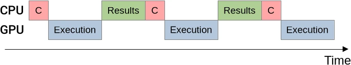
…where “C” stands for command buffer recording, “Execution” stands for execution of GPU work (simulation + results downloads) and “Results” stands for CPU-side results processing.

Command buffer recording has been purposely abbreviated on this diagram as it is expected to be faster than the other two steps, whose relative performance will depends on runtime configuration (relative speed of the GPU and storage device, number of simulation steps per output image…).

In this chapter, we will see how we can make more of these steps happen in parallel.

Command recording

Theory

Because command recording is fast with respect to command execution, allowing them to happen in parallel is not going to save much time. But it will be an occasion to introduce some optimization techniques, that we will later apply on a larger scale to achieve the more ambitious goal of overlapping GPU operations with CPU result processing.

First of all, by looking back at the main simulation loop above, it should be clear to you that it is not possible for the recording of the first command buffer to happen in parallel with its execution. We cannot execute a command buffer that it is still in the process of being recorded.

What we can do, however, is change the logic of our main simulation loop after this first command buffer has been submitted to the GPU:

• Instead of immediately waiting for the GPU to finish the freshly submitted work, we can start preparing a second command buffer on the CPU side while the GPU is busy working on the first command buffer that we just sent.
• Once that second command buffer is ready, we have nothing else to do on the CPU side (for now), so we will just finish executing our first main loop iteration as before: await GPU execution, then process results.
• By the time we reach the second main loop iteration, we will be able to reap the benefits of our optimization by having a second command buffer that can be submitted right away.
• And then the cycle will repeat: we will prepare the command buffer for the third main loop iteration while the GPU work associated with the second main loop iteration is executing, then we will wait, process the second GPU result, and so on.

This sort of ahead-of-time command buffer preparation will result in parallel CPU/GPU execution through pipelining, a general-purpose optimization technique that can improve execution speed at the expense of some duplicated resource allocation and reduced code clarity.

In this particular case, the resource that is being duplicated is the command buffer. Before we used to have only one command buffer in flight at any point in time. Now we intermittently have two of them, one that is being recorded while another one is executing.

And in exchange for this resource duplication, we expect to get a new execution timeline…

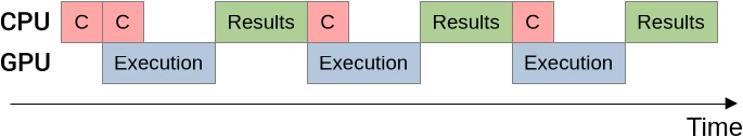
…where command buffer recording and GPU work execution can run in parallel as long as the simulation produces at least two images, resulting in a small performance gain.

Implementation

The design of the SimulationRunner, introduced in the previous chapter, allows us to implement this pipelining optimization through a small modification of our run_simulation() main loop:

// Prepare the first command buffer
let mut cmdbuf = Some(runner.schedule_next_output()?);

// Produce the requested amount of concentration tables
let num_output_images = options.num_output_images;
for image_idx in 0..num_output_images {
    // Submit the command buffer to the GPU and prepare to wait for it
    let future = cmdbuf
        .take()
        .expect("if this iteration executes, a command buffer should be present")
        .execute(context.queue.clone())?
        .then_signal_fence_and_flush()?;

    // Prepare the next command buffer, if any
    if image_idx != num_output_images - 1 {
        cmdbuf = Some(runner.schedule_next_output()?);
    }

    // Wait for the GPU to be done
    future.wait(None)?;

    // Process the simulation output, if enabled
    runner.process_output()?;
}

How does this work?

• Before we begin the main simulation loop, we initialize the simulation pipeline by building a first command buffer, which we do not submit to the GPU right away.
• On each simulation loop iteration, we submit a previously prepared command buffer to the GPU. But in contrast with our previous logic, we do not wait for it right away. Instead, we prepare the next command buffer (if any) while the GPU is executing work.
• Submitting a command buffer to the GPU moves it away, and the static analysis within the Rust compiler that detects use-after-move is unfortunately too simple to understand that we are always going to put another command buffer in its place before the next loop iteration, if there is a next loop iteration. We must therefore play a little trick with the Option type in order to convince the compiler that our code is correct:
  • At first, we wrap our initial command buffer into Some(), thus turning what was an Arc<PrimaryAutoCommandBuffer> into an Option<Arc<PrimaryAutoCommandBuffer>>.
  • When the time comes to submit a command buffer to the GPU, we use the take() method of the Option type to retrieve our command buffer, leaving a None in its place.
  • We then use expect() on the resulting Option to assert that we know it previously contained a command buffer, rather than a None.
  • Finally, when we know that there is going to be a next loop iteration, we prepare the associated command buffer and put it back in the cmdbuf option variable.

While this trick may sound expensive from a performance perspective, you must understand that…

• The Rust compiler’s LLVM backend is a bit more clever than its use-after-move detector, and therefore likely to figure this out and optimize out the Option checks.
• Even if LLVM does not manage, it is quite unlikely that the overhead of checking a boolean flag (testing if an Option is Some) will have any meaningful performance impact compared to the surrounding overhead of scheduling GPU work.

Conclusion

After this coding interlude, we are ready to reach some preliminary conclusions:

• Pipelining is an optimization that can be applied when a computation has two steps A and B that execute on different hardware, and step A produces an output that step B consumes.
• Pipelining allows you to run steps A and B in parallel, at the expense of…
  • Needing to juggle with multiple copies of the output of step A (which will typically come at the expense of a higher application memory footprint).
  • Having a more complex initialization procedure before your main loop, in order to bring your pipeline to the fully initialized state that your main loop expects.
  • Needing some extra logic to avoid unnecessary work at the end of the main loop, if you have real-world use cases where the number of main loop iterations is small enough that this extra work has measurable overhead.

As for performance benefits, you have been warned at the beginning of this section that command buffer recording is only pipelined here because it gives you an easy introduction to this pipelining, and not because the author considers it to be worthwhile.

And indeed, even in a best-case microbenchmarking scenario, the asymptotic performance benefit will be below our performance measurements’ sensitivity threshold…

run_simulation/workgroup16x16/domain2048x1024/total512/image1/compute
                        time:   [136.74 ms 137.80 ms 138.91 ms]
                        thrpt:  [7.7300 Gelem/s 7.7921 Gelem/s 7.8527 Gelem/s]
                 change:
                        time:   [-3.2317% -1.4858% +0.3899%] (p = 0.15 > 0.05)
                        thrpt:  [-0.3884% +1.5082% +3.3396%] No change in
                        performance detected.

Still, this pipelining optimization does not harm much either, and serves as a gateway to more advanced ones. So we will keep it for now.

Results processing

Theory

Encouraged by the modest but tangible performance improvements that pipelined command buffer recording brought, you may now try to achieve full CPU/GPU execution pipelining, in which GPU-side work execution and CPU-side results processing can overlap…

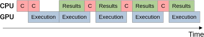
…but your first attempt will likely end with a puzzling compile-time or run-time error, which you will stare at blankly for a few minutes of incomprehension, before you figure it out and thank rustc or vulkano for saving you from yourself.

Indeed there is a trap with this form of pipelining, and one that is easy to fall into: if you are not careful, you are likely to end up trying to access a simulation result on the CPU side, that the GPU could be simultaneously overwriting with a newer result at the same time. Which is the textbook example of a variety of undefined behavior known as a data race.

To avoid this data race, we will need to add double buffering to our CPU-side VBuffer abstraction¹, so that our CPU code can read result N at the same time as our GPU code is busy producing result N+1 and transferring it to the CPU side. And the logic behind our main simulation loop is going to become a bit more complicated again, as we now need to…

• Make sure that by the time we enter the main simulation loop, a result is already available or in the process of being produced. Indeed, the clearest way to write pipelined code is to write each iteration of our main loop under the assumption that the pipeline is already operating at full capacity, taking any required initialization step to get there before the looping begins.
• Rethink our CPU-GPU synchronization strategy so that the CPU code waits for a GPU result to be available before processing it, but does not start processing a result before having scheduled the production of the next result.

Double-buffered VBuffer

As mentioned above, we are going to need some double-buffering inside of VBuffer, which we are therefore going to rename to VBuffers. By now, you should be familiar with the basics of this pattern: we duplicate data storage and add a data member whose purpose is to track the respective role of each of our two buffers…

/// CPU-accessible double buffer used to download the V species' concentration
pub struct VBuffers {
    /// Buffers in which GPU data will be downloaded
    buffers: [Subbuffer<[Float]>; 2],

    /// Truth the the second buffer of the `buffers` array should be used
    /// for the next GPU-to-CPU download
    current_is_1: bool,

    /// Number of columns in the 2D concentration table, including zero padding
    padded_cols: usize,
}
//
impl VBuffers {
    /// Set up `VBuffers`
    pub fn new(options: &RunnerOptions, context: &Context) -> Result<Self> {
        use vulkano::memory::allocator::MemoryTypeFilter as MTFilter;
        let padded_rows = padded(options.num_rows);
        let padded_cols = padded(options.num_cols);
        let new_buffer = || {
            Buffer::new_slice(
                context.mem_allocator.clone(),
                BufferCreateInfo {
                    usage: BufferUsage::TRANSFER_DST,
                    ..Default::default()
                },
                AllocationCreateInfo {
                    memory_type_filter: MTFilter::PREFER_HOST | MTFilter::HOST_RANDOM_ACCESS,
                    ..Default::default()
                },
                (padded_rows * padded_cols) as DeviceSize,
            )
        };
        Ok(Self {
            buffers: [new_buffer()?, new_buffer()?],
            padded_cols,
            current_is_1: false,
        })
    }

    /// Buffer where data has been downloaded two
    /// [`schedule_download_and_flip()`] calls ago, and where data will be
    /// downloaded again on the next [`schedule_download_and_flip()`] call.
    ///
    /// [`schedule_download_and_flip()`]: Self::schedule_download_and_flip
    fn current_buffer(&self) -> &Subbuffer<[Float]> {
        &self.buffers[self.current_is_1 as usize]
    }

    // [ ... more methods coming up ... ]
}

…and then we need to think about when we should alternate between our two buffers. As a reminder, back when it contained a single buffer, the VBuffer type exposed two methods:

• schedule_download(), which prepared a GPU command whose purpose is to transfer the current GPU V concentration input to the VBuffer.
• process(), which was called after the previous command was done executing, and took care of executing CPU post-processing work.

Between the points where these two methods are called, a VBuffer could be not used because it was in the process of being overwritten by the GPU. Which, if we transpose this to our new double-buffered design, sounds like a good point to flip the roles of our two buffers: while the GPU is busy writing to one of the internal buffers, we can do something else with the other buffer:

impl VBuffers {
    [ ... ]

    /// Schedule a download of some [`Concentrations`]' current V input into
    /// [`current_buffer()`](Self::current_buffer), then switch to the other
    /// internal buffer.
    ///
    /// Intended usage is...
    ///
    /// - Schedule two simulation updates and output downloads,
    ///   keeping around the associated futures F1 and F2
    /// - Wait for the first update+download future F1
    /// - Process results on the CPU using [`process()`](Self::process)
    /// - Schedule the next update+download, yielding a future F3
    /// - Wait for F2, process results, schedule F4, etc
    pub fn schedule_download_and_flip(
        &mut self,
        source: &Concentrations,
        cmdbuild: &mut CommandBufferBuilder,
    ) -> Result<()> {
        cmdbuild.copy_buffer(CopyBufferInfo::buffers(
            source.current_inout().input_v.clone(),
            self.current_buffer().clone(),
        ))?;
        self.current_is_1 = !self.current_is_1;
        Ok(())
    }

    [ ... ]
}

As the doc comment indicates, we can use schedule_download_and_flip() method as follows…

1. Schedule a first and second GPU update in short succession
   • Both buffers are now in use by the GPU
   • current_buffer() points to the buffer V1 that is undergoing the first GPU update and will be ready for CPU processing first.
2. Wait for the first GPU update to finish.
   • Cuffent buffer V1 is now ready for CPU readout.
   • Buffer V2 is still being processed by the GPU.
3. Perform CPU-side processing on the current buffer V1.
4. We don’t need V1 anymore after this is done, so schedule a third GPU update.
   • current_buffer() now points to buffer V2, which is still undergoing the second GPU update we scheduled.
   • Buffer V1 is now being processed by the third GPU update.
5. Wait for the second GPU update to finish.
   • Current buffer V2 is now ready for CPU readout.
   • Buffer V1 is still being processed by the third GPU update.
6. We are now back at step 3 but with the roles of V1 and V2 reversed. Repeat steps 3 to 5, reversing the roles of V1 and V2 each time, until all desired outputs have been produced.

…which means that the logic of process() function will basically not change, aside from the fact that it will now use the current_buffer() instead of the former single internal buffer:

impl VBuffers {
    [ ... ]

    /// Process the latest download of the V species' concentrations
    ///
    /// See [`schedule_download_and_flip()`] for intended usage.
    ///
    /// [`schedule_download_and_flip()`]: Self::schedule_download_and_flip
    pub fn process(&self, callback: impl FnOnce(ArrayView2<Float>) -> Result<()>) -> Result<()> {
        // Access the underlying dataset as a 1D slice
        let read_guard = self.current_buffer().read()?;

        // Create an ArrayView2 that covers the whole data, padding included
        let padded_cols = self.padded_cols;
        let padded_elements = read_guard.len();
        assert_eq!(padded_elements % padded_cols, 0);
        let padded_rows = padded_elements / padded_cols;
        let padded_view = ArrayView::from_shape([padded_rows, padded_cols], &read_guard)?;

        // Extract the central region of padded_view, excluding padding
        let data_view = padded_view.slice(s!(
            PADDING_PER_SIDE..(padded_rows - PADDING_PER_SIDE),
            PADDING_PER_SIDE..(padded_cols - PADDING_PER_SIDE),
        ));

        // We are now ready to run the user callback
        callback(data_view)
    }
}

Simulation runner changes

Within the implementation of SimulationRunner, our OutputHandler struct which governs simulation output downloads must now be updated to contain VBuffers instead of a VBuffer…

/// State associated with output downloads and post-processing, if enabled
struct OutputHandler<ProcessV> {
    /// CPU-accessible location to which GPU outputs should be downloaded
    v_buffers: VBuffers,

    /// User-defined post-processing logic for this CPU data
    process_v: ProcessV,
}

…and the SimulationRunner::new() constructor of must be adjusted accordingly.

impl<'run_simulation, ProcessV> SimulationRunner<'run_simulation, ProcessV>
where
    ProcessV: FnMut(ArrayView2<Float>) -> Result<()>,
{
    /// Set up the simulation
    fn new(
        options: &'run_simulation RunnerOptions,
        context: &'run_simulation Context,
        process_v: Option<ProcessV>,
    ) -> Result<Self> {
        // [ ... ]

        // Set up the logic for post-processing V concentration, if enabled
        let output_handler = if let Some(process_v) = process_v {
            Some(OutputHandler {
                v_buffers: VBuffers::new(options, context)?,
                process_v,
            })
        } else {
            None
        };

        // [ ... ]
    }

    // [ ... ]
}

But that is the easy part. The slightly harder part is that in order to achieved the desired degree of pipelining, we should revise the responsibility of the scheduler_download_and_flip() method so that instead of simply building a command buffer, it also submits it to the GPU for eager execution:

impl<'run_simulation, ProcessV> SimulationRunner<'run_simulation, ProcessV>
where
    ProcessV: FnMut(ArrayView2<Float>) -> Result<()>,
{
    // [ ... ]

    /// Submit a GPU job that will produce the next simulation output
    fn schedule_next_output(&mut self) -> Result<FenceSignalFuture<impl GpuFuture + 'static>> {
        // Schedule a number of simulation steps
        schedule_simulation(
            self.options,
            &self.pipelines,
            &mut self.concentrations,
            &mut self.cmdbuild,
        )?;

        // Schedule a download of the resulting V concentration, if enabled
        if let Some(handler) = &mut self.output_handler {
            handler
                .v_buffers
                .schedule_download_and_flip(&self.concentrations, &mut self.cmdbuild)?;
        }

        // Extract the old command buffer builder, replacing it with a blank one
        let old_cmdbuild =
            std::mem::replace(&mut self.cmdbuild, command_buffer_builder(self.context)?);

        // Build the command buffer and submit it to the GPU
        let future = old_cmdbuild
            .build()?
            .execute(self.context.queue.clone())?
            .then_signal_fence_and_flush()?;
        Ok(future)
    }

    // [ ... ]
}

…and being nice people, we should also warn users of the process_output() that although its implementation has not changed much, its usage contract has become more complicated:

impl<'run_simulation, ProcessV> SimulationRunner<'run_simulation, ProcessV>
where
    ProcessV: FnMut(ArrayView2<Float>) -> Result<()>,
{
    // [ ... ]

    /// Process the simulation output, if enabled
    ///
    /// This method is meant to be used in the following way:
    ///
    /// - Initialize the simulation pipeline by submitting two simulation jobs
    ///   using [`schedule_next_output()`](Self::schedule_next_output)
    /// - Wait the first simulation job to finish executing
    /// - Call this method to process the output of the first job
    /// - Submit a third simulation job
    /// - Wait the second simulation job to finish executing
    /// - Call this method to process the output of the second job
    /// - ...and so on, until all simulation outputs have been processed...
    fn process_output(&mut self) -> Result<()> {
        if let Some(handler) = &mut self.output_handler {
            handler.v_buffers.process(&mut handler.process_v)?;
        }
        Ok(())
    }
}

Once this is done, migrating run_simulation() to the new pipelined logic becomes straightforward:

/// Simulation runner, with a user-specified output processing function
pub fn run_simulation<ProcessV: FnMut(ArrayView2<Float>) -> Result<()>>(
    options: &RunnerOptions,
    context: &Context,
    process_v: Option<ProcessV>,
) -> Result<()> {
    // Set up the simulation
    let mut runner = SimulationRunner::new(options, context, process_v)?;

    // Schedule the first simulation update
    let mut current_future = Some(runner.schedule_next_output()?);

    // Produce the requested amount of concentration tables
    let num_output_images = options.num_output_images;
    for image_idx in 0..num_output_images {
        // Schedule the next simulation update, if any
        let next_future = (image_idx < num_output_images - 1)
            .then(|| runner.schedule_next_output())
            .transpose()?;

        // Wait for the GPU to be done with the previous update
        current_future
            .expect("if this loop iteration executes, a future should be present")
            .wait(None)?;
        current_future = next_future;

        // Process the simulation output, if enabled
        runner.process_output()?;
    }
    Ok(())
}

As previously hinted, this is quite similar to the previosu logic where we used to prepare a new command buffer while the previous command buffer is executing, except now we take it further and submit a full GPU job while another full GPU job is already executing.

And as before, some tricks must be played with Option in order to convince the Rust compiler’s borrow checker that even though we do not schedule a new computation on the last loop iteration, our inner Option of FenceSignalFuture will always be Some() or we’ll die at runtime, and therefore use-after-move of GPU futures cannot happen.

Exercise

Implement the pipelining techniques described above, then adapt the simulation executable and benchmark, and check the impact on performance.

You should observe a noticeable performance improvement when running the main simulation binary over a fast storage device like /dev/shm, as the previous version of the simulation spent too much time keeping waiting for the GPU to keep this storage device busy.

Microbenchmarks will see more modest performance improvements except for compute+download+sum, which will see a great improvement in scenarios that produce many concentration tables because its CPU post-processing can now run in parallel with GPU work.

1. Another example of how pipelining requires duplication of (in this case memory) resources. ↩

Async download

Introduction

During the last chapter, we set up the required pipelining infrastructure for the CPU and GPU steps of computation to execute in parallel with each other. This took us from a situation where the CPU and GPU kept waiting for each other…

…to a situation where it is only the fastest device that awaits the slowest device:

However, the above diagrams are simplifications of a more complex hardware reality, where both the CPU and GPU work are composed of many independent components that can operate in parallel. By introducing more parallelism on either side, we should be able to improve our performance further. But how should we focus this effort?

On the CPU side, we mentioned multiple times that command buffer recording is relatively cheap. Which means we do not expect a massive performance benefit from offloading it to a different thread, and because of thread synchronization costs it could be a net loss. Beyond that, the other CPU tasks that we could consider parallelizing are all IO-related:

• NVMe storage and ramdisks like /dev/shm are fast enough to benefit from the use of multiple I/O threads. But unfortunately the HDF5 library does not know how to correctly leverage multithreading for I/O, so we are stuck with our choice of file format here.
• What we do control is the copy of GPU results from the main CPU thread to the I/O thread, which is currently performed in a sequential manner. But parallelizing memory-bound tasks like this is rather difficult, and we only expect significant benefits in I/O bound worloads that write to a ramdisk, which are arguably a bit of an edge case.

Taking all this into consideration, further CPU-side parallelization does not look very promising at this point. But what about GPU-side parallelization? That’s a deep topic, so in this chapter we will start with the first stage of GPU execution, which is the submission of commands from the CPU.

Right from this stage, a typical high-end modern GPU provides at least 2-3 flavors of independent hardware command submission interfaces, which get exposed as queue families in Vulkan:

• “Main” queues support all operations including traditional live 3D rendering.
• “Asynchronous compute” queues can execute compute commands and data transfer operations in parallel with the main queues when enough resources are available.
• Dedicated “DMA” queues, if available, can only execute data transfer commands but have a higher chance to be able to operate in parallel with the other queues.

Knowing this, we would now like to leverage this extra hardware parallelism, if available, in order to go from our current sequential GPU execution model…

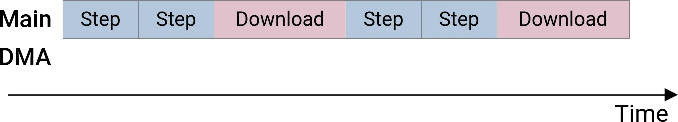
…to a state that leverages the hardware concurrent data transfer capabilities if available:

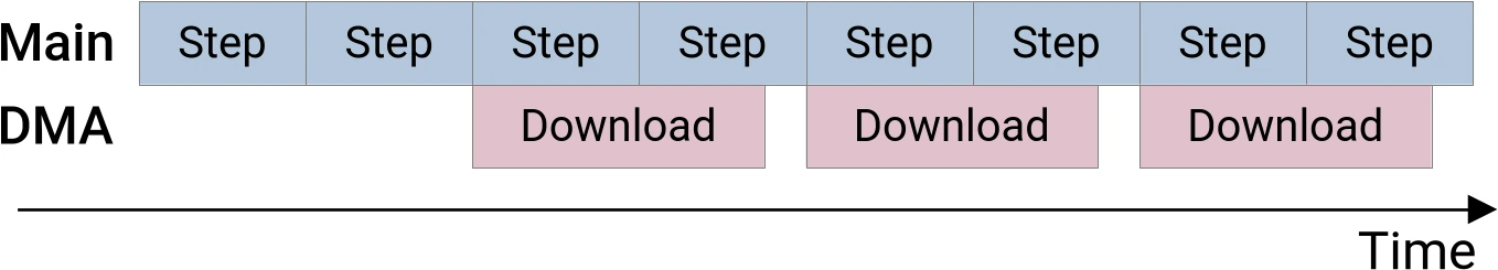
The purpose of this chapter will be to take us from here to there. From this optimization, we expect to improve the simulation’s performance by up to 2x in the best-case scenario where computation steps and GPU-to-CPU data transfers take roughly the same amount of time, and the application performance is limited by the speed at which the GPU does its work (as opposed to e.g. the speed at which data gets written to a storage device).

Transfer queue

To perform asynchronous data transfers, the first thing that we are going to need is some access to the GPU’s dedicated DMA (if available) or asynchronous compute queues.¹ To get there, we will need to break an assumption that has been hardcoded in our codebase for a while, namely that a single Queue ought to be enough for anybody.

The first step in this journey will be for us to rename our queue family selection function to highlight its compute-centric nature:

fn compute_queue_family_index(device: &PhysicalDevice) -> u32 {
    device
        .queue_family_properties()
        .iter()
        .position(|family| family.queue_flags.contains(QueueFlags::COMPUTE))
        .expect("device does not support compute (or graphics)") as u32
}

We will then write a second version of this function that attempts to pick up the device’s dedicated DMA queue (if available) or its asynchronous compute queue (otherwise). This is hard to do in a hardware-agnostic way, but one fairly reliable trick is to pick the queue family that supports data transfers and as few other Vulkan operations as possible:

/// Pick up the queue family that has the highest chance of supporting
/// asynchronous data transfers, and is distinct from the main compute queue
fn transfer_queue_family_index(device: &PhysicalDevice, compute_idx: u32) -> Option<u32> {
    use QueueFlags as QF;
    device
        .queue_family_properties()
        .iter()
        .enumerate()
        .filter(|(idx, family)| {
            // Per the Vulkan specification, if a queue family supports graphics
            // or compute, then it is guaranteed to support data transfers and
            // does not need to advertise support for it. Why? Ask Khronos...
            *idx != compute_idx as usize
                && family
                    .queue_flags
                    .intersects(QF::TRANSFER | QF::COMPUTE | QF::GRAPHICS)
        })
        .min_by_key(|(idx, family)| {
            // Among the queue families that support data transfers, we priorize
            // the queue families that...
            //
            // - Explicitly advertise support for data transfers
            // - Advertise support for as few other operations as possible
            // - Come as early in the queue family list as possible
            let flags = family.queue_flags;
            let flag_priority = if flags.contains(QF::TRANSFER) { 0 } else { 1 };
            let specialization = flags.count();
            (flag_priority, specialization, *idx)
        })
        .map(|(idx, _family)| idx as u32)
}

We will then modify our device setup code to allocate one queue from each of these families…

/// Initialized `Device` with associated queues
struct DeviceAndQueues {
    device: Arc<Device>,
    compute_queue: Arc<Queue>,
    transfer_queue: Option<Arc<Queue>>,
}
//
impl DeviceAndQueues {
    /// Set up a device and associated queues
    fn new(device: Arc<PhysicalDevice>) -> Result<Self> {
        // Prepare to request queues
        let mut queue_create_infos = Vec::new();
        let queue_create_info = |queue_family_index| QueueCreateInfo {
            queue_family_index,
            ..Default::default()
        };

        // Create a compute queue, and a transfer queue if distinct
        let compute_family = compute_queue_family_index(&device);
        queue_create_infos.push(queue_create_info(compute_family));
        if let Some(transfer_family) = transfer_queue_family_index(&device, compute_family) {
            queue_create_infos.push(queue_create_info(transfer_family))
        }

        // Set up the device and queues
        let (device, mut queues) = Device::new(
            device,
            DeviceCreateInfo {
                queue_create_infos,
                ..Default::default()
            },
        )?;

        // Get the compute queue, and the transfer queue if available
        let compute_queue = queues
            .next()
            .expect("we asked for a compute queue, we should get one");
        let transfer_queue = queues.next();
        Ok(Self {
            device,
            compute_queue,
            transfer_queue,
        })
    }
}

…and finally, we are going to integrate this new nuance into our context struct.

/// Basic Vulkan setup that all our example programs will share
pub struct Context {
    pub device: Arc<Device>,
    pub compute_queue: Arc<Queue>,
    pub transfer_queue: Option<Arc<Queue>>,
    pipeline_cache: PersistentPipelineCache,
    pub mem_allocator: Arc<MemoryAllocator>,
    pub desc_allocator: Arc<DescriptorSetAllocator>,
    pub comm_allocator: Arc<CommandBufferAllocator>,
    _messenger: Option<DebugUtilsMessenger>,
}
//
impl Context {
    /// Set up a `Context`
    pub fn new(
        options: &ContextOptions,
        quiet: bool,
        progress: Option<ProgressBar>,
    ) -> Result<Self> {
        let library = VulkanLibrary::new()?;
        let mut logging_instance = LoggingInstance::new(library, &options.instance, progress)?;
        let physical_device =
            select_physical_device(&logging_instance.instance, &options.device, quiet)?;
        let DeviceAndQueues {
            device,
            compute_queue,
            transfer_queue,
        } = DeviceAndQueues::new(physical_device)?;
        let pipeline_cache = PersistentPipelineCache::new(device.clone())?;
        let (mem_allocator, desc_allocator, comm_allocator) = setup_allocators(device.clone());
        let _messenger = logging_instance.messenger.take();
        Ok(Self {
            device,
            compute_queue,
            transfer_queue,
            pipeline_cache,
            mem_allocator,
            desc_allocator,
            comm_allocator,
            _messenger,
        })
    }

    // [ ... same as before ... ]
}

After this is done, we can let compiler errors guide us into replacing every occurence of context.queue in our program with context.compute_queue. And with that, we will get a program that still only uses a single Vulkan compute queue… but now possibly allocates another data transfer queue that we will be able to leverage next.

Triple buffering

Theory

Having reached the point where we do have access to a data transfer queue, we could proceed to adjust our command buffer creation and queue submission logic to perform asynchronous data transfers. But then we would once again get a rustc or vulkano error, get puzzled by that error, think it through, and after a while thank these tools for saving us from ourselves again.

Indeed, asynchronous data transfers are yet another application on the general concept of pipelining optimizations. And like all pipelining optimizations, they require some kind of resource duplication in order to work. Without such duplication, we will once again face a data race:

In case the above diagram does not make it apparent, the problem with our current memory management strategy is that if we try to download the UV1 version of the V species’ concentration while running more simulation steps, and our download takes more time than one simulation step, then subsequent simulation steps will eventually end up overwriting the data that we are in the process of transfering to the CPU, resulting in yet another data race.

We can avoid this data race by allocating a third set of (U, V) concentrations buffers on the GPU side. Which will allow us to have not just one, but three pairs of (U, V) datasets, where each pair does not contain one of the three (U, V) datasets…

• The (UV2, UV3) pair does not contain UV1
• The (UV1, UV3) pair does not contain UV2
• The (UV1, UV2) pair does not contain UV3

…and thus, by leveraging each of these pairs at the right time during our simulation steps, we will be able to keep computing new simulation steps on the GPU without overwriting the version of the (U, V) concentration data that is in the process of being transferred to the CPU side:

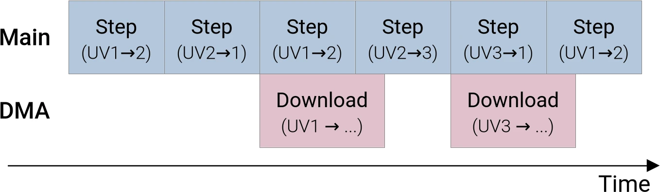
But needless to say, getting there will require us to make “a few” changes to the logic that we use to manage our GPU-side concentration data storage. Which will be the topic of the next section.

Implementation

Previously, our Concentrations type was effectively a double buffer of InOut, where each InOut contained a Vulkan descriptor set (for compute pipeline execution purposes) and a V input buffer (for output downloading purposes).

Now that we are doing triple buffering, however, we would need to have six such InOut structs, with redundant V input buffers, and that starts to feel wasteful. So instead of doing that, we will extract the descriptor set setup logic out of InOut…

/// Set up a descriptor set that uses a particular `(U, V)` dataset as
/// inputs and another `(U, V)` dataset as outputs
fn setup_descriptor_set(
    context: &Context,
    layout: &PipelineLayout,
    in_u: Subbuffer<[Float]>,
    in_v: Subbuffer<[Float]>,
    out_u: Subbuffer<[Float]>,
    out_v: Subbuffer<[Float]>,
) -> Result<Arc<DescriptorSet>> {
    // Determine how the descriptor set will bind to the compute pipeline
    let set_layout = layout.set_layouts()[INOUT_SET as usize].clone();

    // Configure what resources will attach to the various bindings
    // that the descriptor set is composed of
    let descriptor_writes = [
        WriteDescriptorSet::buffer_array(IN, 0, [in_u, in_v]),
        WriteDescriptorSet::buffer_array(OUT, 0, [out_u, out_v]),
    ];

    // Set up the descriptor set according to the above configuration
    let descriptor_set = DescriptorSet::new(
        context.desc_allocator.clone(),
        set_layout,
        descriptor_writes,
        [],
    )?;
    Ok(descriptor_set)
}

…and trash the rest of InOut, replacing it with a new DoubleUV struct that is just a double buffer of descriptor sets that does not even handle buffer allocation duties anymore:

/// Double-buffered chemical species concentration storage
///
/// This manages Vulkan descriptor sets associated with a pair of `(U, V)`
/// chemical concentrations datasets, such that...
///
/// - At any point in time, one `(U, V)` dataset serves as inputs to the active
///   GPU compute pipeline, and another `(U, V)` dataset serves as outputs.
/// - A normal simulation update takes place by calling the
///   [`update()`](Self::update) method, which invokes a user-specified callback
///   with the descriptor set associated with the current input/output
///   configuration, then flips the role of the buffers (inputs become outputs
///   and vice versa).
/// - The [`current_descriptor_set()`](Self::current_descriptor_set) method can be used to query the
///   current descriptor set _without_ flipping the input/output roles. This is
///   useful for the triple buffering logic discussed below.
struct DoubleUV {
    /// If we denote `(U1, V1)` the first `(U, V)` concentration dataset and
    /// `(U2, V2)` the second concentration dataset...
    ///
    /// - The first "forward" descriptor set uses `(U1, V1)` as its inputs and
    ///   `(U2, V2)` as its outputs.
    /// - The second "reverse" descriptor set uses `(U2, V1)` as its inputs and
    ///   `(U2, V2)` as its outputs.
    descriptor_sets: [Arc<DescriptorSet>; 2],

    /// Truth that the "reverse" descriptor set is being used
    reversed: bool,
}
//
impl DoubleUV {
    /// Set up a `DoubleUV`
    fn new(
        context: &Context,
        layout: &PipelineLayout,
        u1: Subbuffer<[Float]>,
        v1: Subbuffer<[Float]>,
        u2: Subbuffer<[Float]>,
        v2: Subbuffer<[Float]>,
    ) -> Result<Self> {
        let forward = setup_descriptor_set(
            context,
            layout,
            u1.clone(),
            v1.clone(),
            u2.clone(),
            v2.clone(),
        )?;
        let reverse = setup_descriptor_set(context, layout, u2, v2, u1, v1)?;
        Ok(Self {
            descriptor_sets: [forward, reverse],
            reversed: false,
        })
    }

    /// Currently selected descriptor set
    fn current_descriptor_set(&self) -> Arc<DescriptorSet> {
        self.descriptor_sets[self.reversed as usize].clone()
    }

    /// Run a simulation step and flip the input/output roles
    fn update(&mut self, step: impl FnOnce(Arc<DescriptorSet>) -> Result<()>) -> Result<()> {
        step(self.current_descriptor_set())?;
        self.reversed = !self.reversed;
        Ok(())
    }
}

All the complexity of triple buffering will be handled by the top-level Concentrations struct, which is the only one that has all the information needed to take correct triple-buffering decisions. As the associated logic is sophisticated, we will help maintenance with an fair amount of doc comments:

/// Triple-buffered chemical species concentration storage
///
/// This manages three `(U, V)` chemical concentration datasets in such a way
/// that the following properties are guaranteed:
///
/// - At any point in time, a normal simulation update can be performed using
///   the [`update()`] method. This method will...
///   1. Invoke a user-specified callback with a descriptor set that goes from
///      one of the inner `(U, V)` datasets (let's call it `(Ui, Vi)`) to
///      another dataset (let's call it `(Uj, Vj)`).
///   2. Update the `Concentrations` state in such a way that the next time
///      [`update()`] is called, the descriptor set that will be provided will
///      use the former output dataset (called `(Uj, Vj)` above) as its input,
///      and another dataset as its output (can either be the same `(Ui, Vi)`
///      dataset used as input above, or the third `(Uk, Vk)` dataset).
/// - At any point in time, the [`lock_current_v()`](Self::lock_current_v)
///   method can be called as a preparation for downloading the current V
///   species concentration. This method will...
///   1. Return the [`Subbuffer`] associated with the current V species
///      concentration, i.e. the buffer that the next [`update()`] call will use
///      as its V concentration input.
///   2. Update the `Concentrations` state in such a way that subsequent calls
///      to [`update()`] will not use this buffer as their V species
///      concentration output. The other two `(U, V)` datasets will be used in a
///      double-buffered fashion instead.
///
/// The underlying logic assumes that the user will wait for the current data
/// download to complete before calling `lock_current_v()` again.
///
/// [`update()`]: Self::update
pub struct Concentrations {
    /// `Vi` buffer from each of the three `(Ui, Vi)` datasets that we manage.
    v_buffers: [Subbuffer<[Float]>; 3],

    /// Double buffers that leverage a pair of `(U, V)` datasets, such that the
    /// double buffer at index `i` within this array **does not** use the `(Ui,
    /// Vi)` dataset per the `v_buffers` indexing convention.
    ///
    /// For example, the double buffer at index 1 does not use the `(U1, V1)`
    /// dataset, it alternates between the `(U0, V0)` and `(U2, V2)` datasets.
    double_buffers: [DoubleUV; 3],

    /// Currently selected entry of `double_buffers`, used for `update()` calls
    /// after any `transitional_set` has been taken care of.
    double_buffer_idx: usize,

    /// Descriptor set used to perform the transition between two entries of the
    /// `double_buffers` array.
    ///
    /// Most of the time, simulation updates are fully managed by one
    /// [`DoubleUV`], i.e. they keep going from one `(Ui, Vi)` dataset to
    /// another `(Uj, Vj)` dataset and back, while the third `(Uk, Vk)` dataset
    /// is unused. However, when [`lock_current_v()`] gets called...
    ///
    /// - If we denote `(Ui, Vi)` the dataset currently used as input, it must
    ///   not be modified as long as the download scheduled by
    ///   [`lock_current_v()`] is ongoing. Therefore, the next simulation
    ///   updates must be performed using another double buffer composed of the
    ///   other two `(Uj, Vj)` and `(Uk, Vk)` datasets.
    /// - Before this can happen, we need to take one simulation step that uses
    ///   `(Ui, Vi)` as input and one of `(Uj, Vj)` or `(Uk, Vk)` as output, so
    ///   that one of these can become the next simulation input.
    ///
    /// `transitional_set` is the descriptor set that is used to perform the
    /// simulation step described above, before we can switch back to our
    /// standard double buffering logic.
    ///
    /// [`lock_current_v()`]: Self::lock_current_v
    transitional_set: Option<Arc<DescriptorSet>>,
}

The implementation of this new Concentrations struct starts with the buffer allocation stage, which is largely unchanged compared to what InOut::allocate_buffers() used to do. We simply allocate 6 buffers instead of 4, because now we need three U storage buffers and three V storage buffers:

impl Concentrations {
    /// Allocate the set of buffers that we are going to use
    fn allocate_buffers(
        options: &RunnerOptions,
        context: &Context,
    ) -> Result<[Subbuffer<[Float]>; 6]> {
        use BufferUsage as BU;
        let padded_rows = padded(options.num_rows);
        let padded_cols = padded(options.num_cols);
        let new_buffer = || {
            Buffer::new_slice(
                context.mem_allocator.clone(),
                BufferCreateInfo {
                    usage: BU::STORAGE_BUFFER | BU::TRANSFER_DST | BU::TRANSFER_SRC,
                    ..Default::default()
                },
                AllocationCreateInfo::default(),
                (padded_rows * padded_cols) as DeviceSize,
            )
        };
        Ok([
            new_buffer()?,
            new_buffer()?,
            new_buffer()?,
            new_buffer()?,
            new_buffer()?,
            new_buffer()?,
        ])
    }

    // [ ... ]
}

The new version of the create_and_schedule_init() constructor will not be that different from its predecessor at a conceptual level. But it will have a few more buffers to initialize, and will also need to set the stage for triple buffering shenanigans to come.

impl Concentrations {
    // [ ... ]

    /// Set up GPU data storage and schedule GPU buffer initialization
    ///
    /// GPU buffers will only be initialized after the command buffer associated
    /// with `cmdbuild` has been built and submitted for execution. Any work
    /// that depends on their initial value must be scheduled afterwards.
    pub fn create_and_schedule_init(
        options: &RunnerOptions,
        context: &Context,
        pipelines: &Pipelines,
        cmdbuild: &mut CommandBufferBuilder,
    ) -> Result<Self> {
        // Allocate all GPU storage buffers used by the simulation
        let [u0, v0, u1, v1, u2, v2] = Self::allocate_buffers(options, context)?;

        // Keep around the three V concentration buffers from these datasets
        let v_buffers = [v0.clone(), v1.clone(), v2.clone()];

        // Set up three (U, V) double buffers such that the double buffer at
        // index i uses the 4 buffers that do not include (Ui, Vi), and the
        // "forward" direction of each double buffer goes from the dataset of
        // lower index to the dataset of higher index.
        let layout = &pipelines.layout;
        let double_buffers = [
            DoubleUV::new(
                context,
                layout,
                u1.clone(),
                v1.clone(),
                u2.clone(),
                v2.clone(),
            )?,
            DoubleUV::new(
                context,
                layout,
                u0.clone(),
                v0.clone(),
                u2.clone(),
                v2.clone(),
            )?,
            DoubleUV::new(context, layout, u0.clone(), v0.clone(), u1, v1)?,
        ];

        // Schedule the initialization of the first simulation input
        //
        // - We will initially work with the double buffer at index 0, which is
        //   composed of datasets (U1, V1) and (U2, V2).
        // - We will initially access it in order, which means that the (U1, V1)
        //   dataset will be the first simulation input.
        // - Due to the above, to initialize this first simulation input, we
        //   need to bind a descriptor set that uses (U1, V1) as its output.
        // - This is true of the reverse descriptor set within the first double
        //   buffer, in which (U2, V2) is the input and (U1, V1) is the output.
        let double_buffer_idx = 0;
        cmdbuild.bind_pipeline_compute(pipelines.init.clone())?;
        cmdbuild.bind_descriptor_sets(
            PipelineBindPoint::Compute,
            pipelines.layout.clone(),
            INOUT_SET,
            double_buffers[double_buffer_idx].descriptor_sets[1].clone(),
        )?;
        let num_workgroups = |domain_size: usize, workgroup_size: NonZeroU32| {
            padded(domain_size).div_ceil(workgroup_size.get() as usize) as u32
        };
        let padded_workgroups = [
            num_workgroups(options.num_cols, options.pipeline.workgroup_cols),
            num_workgroups(options.num_rows, options.pipeline.workgroup_rows),
            1,
        ];
        // SAFETY: GPU shader has been checked for absence of undefined behavior
        //         given a correct execution configuration, and this is one
        unsafe {
            cmdbuild.dispatch(padded_workgroups)?;
        }

        // Any dataset other than the (U1, V1) initial input must have its edges
        // initialized to zeros.
        //
        // Only the edges need to be initialized. The values at the center of
        // the dataset do not matter, as these buffers will serve as simulation
        // outputs at least once (which will initialize their central values)
        // before they serve as a simulation input.
        //
        // Here we initialize the entire buffer to zero, as the Vulkan
        // implementation is likely to special-case this buffer-zeroing
        // operation with a high-performance implementation.
        cmdbuild.fill_buffer(u0.reinterpret(), 0)?;
        cmdbuild.fill_buffer(v0.reinterpret(), 0)?;
        cmdbuild.fill_buffer(u2.reinterpret(), 0)?;
        cmdbuild.fill_buffer(v2.reinterpret(), 0)?;

        // Once the command buffer is executed, everything will be ready
        Ok(Self {
            v_buffers,
            double_buffers,
            double_buffer_idx,
            transitional_set: None,
        })
    }

    // [ ... ]
}

For reasons that will become clear later on, we will drop the idea of having a current_inout() function. Instead, we will only have…

• An update() method that is used when performing simulation steps, as before.
• A new lock_current_v() method that is used when scheduling a V concentration download.

We will describe the latter first, as its internal logic will motivate the existence of the new transitional_set data member of the Concentrations struct, which the update() method will later need to use in an appropriate manner.

As mentioned above, lock_current_v() should be called after scheduling a set of simulation steps, in order to lock the current (U, V) dataset for the duration of the final GPU-to-CPU download. This will prevent the associated V buffer from being used as a simulation output for the duration of the download, and provide the associated Subbuffer to the caller so that it can initiate the download:

impl Concentrations {
    // [ ... ]

    /// Lock the current V species concentrations for a GPU-to-CPU download
    fn lock_current_v(&mut self) -> Subbuffer<[Float]> {
        // [ ... ]
    }

    // [ ... ]
}

The implementation of lock_current_v() starts with a special case which we will not discuss yet, which handles the scenario where two GPU-to-CPU downloads are initiated in quick succession without any simulation step inbetween. After this, we get code for the general case where some simulation steps have occured after the previous GPU-to-CPU download.

First of all, we use the index of the current double buffer and its reversed flag in order to tell what are the index of the current input and output buffer, using the indexing convention introduced by the Concentrations::create_and_schedule_init() constructor:

// [ ... handle special case of two consecutive downloads ... ]

let initial_double_buffer_idx = self.double_buffer_idx;
let (mut initial_input_idx, mut initial_output_idx) = match initial_double_buffer_idx {
    0 => (1, 2),
    1 => (0, 2),
    2 => (0, 1),
    _ => unreachable!("there are only three double buffers"),
};
let initial_double_buffer = &self.double_buffers[initial_double_buffer_idx];
if initial_double_buffer.reversed {
    std::mem::swap(&mut initial_input_idx, &mut initial_output_idx);
}

From this, we trivially deduce which buffer within the Concentrations::v_buffers array is our current V input buffer. We keep a copy of it, that will be the return value of lock_current_v():

let input_v = self.v_buffers[initial_input_idx].clone();

The remainder of lock_current_v()’s implementation will then be concerned with ensuring that this V buffer is not used as a simulation output again as long as a GPU-to-CPU download is in progress. The indexing convention of the Concentrations::double_buffers array has been chosen such that this is just a matter of switching to the double-buffer at index initial_input_idx…

let next_double_buffer_idx = initial_input_idx;

…but before we start using this double buffer, we must first perform a simulation step that takes the simulation input from our current input buffer (which is not part of the new double buffer) to another buffer (which will be part of the new double buffer since there are only three (U, V) pairs).

For example, assuming we are initially using the first double buffer (whose members are datasets (U1, V1) and (U2, V2)) and our current input buffer is (U1, V1), we will want to move to the second double buffer (whose members ars datasets (U0, V0) and (U2, V2)) by performing one simulation step that goes from (U1, V1) to (U0, V0) or (U2, V2).

It should be apparent that the active descriptor set within the current double buffer (which, in the above example, performs a simulation step from dataset (U1, V1) to dataset (U2, V2)) will always go to one of the datasets within the new double buffer, so we can use it to perform the transition…

self.transitional_set = Some(initial_double_buffer.current_descriptor_set().clone());

…but we must then configure the new double buffer’s reversed flag so that the first simulation step that uses it goes in the right direction. In the above example, after the transitional step that uses (U1, V1) as input and (U2, V2) as output, we want to the next simulation step to go from (U2, V2) to (U0, V0), and not from (U0, V0) to (U2, V2).

This can be done by figuring out what will be the index of the input and output datasets in the first step that uses the new double buffer…

let next_input_idx = initial_output_idx;
let next_output_idx = match (next_double_buffer_idx, next_input_idx) {
    (0, 1) => 2,
    (0, 2) => 1,
    (1, 0) => 2,
    (1, 2) => 0,
    (2, 0) => 1,
    (2, 1) => 0,
    _ => {
        unreachable!(
            "there are only three double buffers, each of which has \
            one input and one output dataset whose indices differ from \
            the double buffer's index"
        )
    }
};

…and setting up the reversed flag of the new double buffer accordingly:

self.double_buffer_idx = next_double_buffer_idx;
self.double_buffers[next_double_buffer_idx].reversed = next_output_idx < next_input_idx;

Once the Concentrations is set up in this way, we can return the input_v that we previously recorded to the caller of lock_current_v(). And this is the end of the implementation of the lock_current_v() function.

The update() method’s implementation is then written in such a way that any transitional_step is taken first before using the current double buffer, to make sure that any double buffer transition scheduled by lock_current_v() is performed before the new double buffer is used…

impl Concentrations {
    // [ ... ]

    /// Run a simulation step
    ///
    /// The `step` callback will be provided with the descriptor set that should
    /// be used for the next simulation step. If you need to carry out multiple
    /// simulation steps, you should call `update()` once per simulation step.
    pub fn update(&mut self, step: impl FnOnce(Arc<DescriptorSet>) -> Result<()>) -> Result<()> {
        if let Some(transitional_set) = self.transitional_set.take() {
            // If we need to transition from a freshly locked (U, V) dataset to
            // another double buffer, do so...
            step(transitional_set)
        } else {
            // ...otherwise, keep using the current double buffer
            self.double_buffers[self.double_buffer_idx].update(step)
        }
    }
}

…and because this uses Option::take(), there is a guarantee that the transitional simulation step will only be carried out once. After that, Concentrations will resume using a simple double-buffering logic as it did before the current V buffer was locked.

There is just one edge case to take care of. If two GPU-to-CPU downloads are started in quick succession, with not simulation step inbetween, then all the buffer-locking work has already been carried out by the lock_current_v() call that initiated the first GPU-to-CPU download.

As a result, we do not need to do anything to lock the current input buffer (which has been done already), and can simply figure out the input_v buffer associated with the current V concentration input and return it right away. That’s what the edge case handling at the beginning of lock_current_v() does, completing the implementation of this function:

impl Concentrations {
    // [ ... ]

    /// Lock the current V species concentrations for a GPU-to-CPU download
    fn lock_current_v(&mut self) -> Subbuffer<[Float]> {
        // If no update has been carried out since the last lock_current_v()
        // call, then we do not need to change anything to the current
        // Concentrations state, and can simply return the current V input
        // buffer again. Said input buffer is easily identified as the one that
        // future simulation updates will be avoiding.
        if self.transitional_set.is_some() {
            return self.v_buffers[self.double_buffer_idx].clone();
        }

        // Otherwise, determine the index of the input and output buffer of the
        // currently selected descriptor set
        let initial_double_buffer_idx = self.double_buffer_idx;
        let (mut initial_input_idx, mut initial_output_idx) = match initial_double_buffer_idx {
            0 => (1, 2),
            1 => (0, 2),
            2 => (0, 1),
            _ => unreachable!("there are only three double buffers"),
        };
        let initial_double_buffer = &self.double_buffers[initial_double_buffer_idx];
        if initial_double_buffer.reversed {
            std::mem::swap(&mut initial_input_idx, &mut initial_output_idx);
        }

        // The initial simulation input is going to be downloaded...
        let input_v = self.v_buffers[initial_input_idx].clone();

        // ...and therefore we must refrain from using it as a simulation output
        // in the future, which we do by switching to the double buffer that
        // does not use this dataset (by definition of self.double_buffers)
        let next_double_buffer_idx = initial_input_idx;

        // To perform this transition correctly, we must first perform one
        // simulation step that uses the current dataset as input and another
        // dataset as output. The current descriptor set within the double
        // buffer that we used before does take us from our initial (Ui, Vi)
        // input dataset to another (Uj, Vj) output dataset, and is therefore
        // appropriate for this purpose.
        self.transitional_set = Some(initial_double_buffer.current_descriptor_set().clone());

        // After this step, we will land into a (Uj, Vj) dataset that is part of
        // our new double buffer, but we do not know if it is the first or the
        // second dataset within this double buffer. And we need to know that in
        // order to set the "reversed" flag of the double buffer correctly.
        //
        // We already know what is the index of the dataset that serves as a
        // transitional output, and from that and the index of our new double
        // buffer, we can tell what is the index of the third dataset, i.e. the
        // other dataset within our new double buffer...
        let next_input_idx = initial_output_idx;
        let next_output_idx = match (next_double_buffer_idx, next_input_idx) {
            (0, 1) => 2,
            (0, 2) => 1,
            (1, 0) => 2,
            (1, 2) => 0,
            (2, 0) => 1,
            (2, 1) => 0,
            _ => {
                unreachable!(
                    "there are only three double buffers, each of which has \
                    one input and one output dataset whose indices differ from \
                    the double buffer's index"
                )
            }
        };

        // ...and given that, we can easily tell if the first step within our
        // next double buffer, after the transitional step, will go in the
        // forward or reverse direction.
        self.double_buffer_idx = next_double_buffer_idx;
        self.double_buffers[next_double_buffer_idx].reversed = next_output_idx < next_input_idx;
        input_v
    }

    // [ ... ]
}

VBuffers changes

To be able to use the new version of Concentrations, a couple of changes to the VBuffers::schedule_download_and_flip() method are required:

• This method must now receive &mut Concentrations, not just &Concentrations, as it now needs to modify the Concentrations triple buffering configuration using lock_current_v() instead of simply querying its current input buffer for the V concentration.
• …and the output of lock_current_v() tells it what the current V input buffer is, which is what it needs to initiate the GPU-to-CPU download.

Overall, the new implementation looks like this:

pub fn schedule_download_and_flip(
    &mut self,
    source: &mut Concentrations,
    cmdbuild: &mut CommandBufferBuilder,
) -> Result<()> {
    cmdbuild.copy_buffer(CopyBufferInfo::buffers(
        source.lock_current_v(),
        self.current_buffer().clone(),
    ))?;
    self.current_is_1 = !self.current_is_1;
    Ok(())
}

Simulation runner changes

Now that our data management infrastructure is ready for concurrent computations and GPU-to-CPU downloads, the last part of the work is to update our top-level simulation scheduling logic so that it actually uses a dedicated data transfer queue (if available) to run simulation steps and GPU-to-CPU data transfers concurrently.

To do this, we must first generalize our command buffer builder constructor so that it can work with any queue, not just the compute queue.

fn command_buffer_builder(context: &Context, queue: &Queue) -> Result<CommandBufferBuilder> {
    let cmdbuild = CommandBufferBuilder::primary(
        context.comm_allocator.clone(),
        queue.queue_family_index(),
        CommandBufferUsage::OneTimeSubmit,
    )?;
    Ok(cmdbuild)
}

Then we modify the definition of SimulationRunner to clarify that its internal command buffer builder is destined to host compute queue operations only…

/// State of the simulation
struct SimulationRunner<'run_simulation, ProcessV> {
    // [ ... members other than "cmdbuild" are unchanged ... ]

    /// Next command buffer to be executed on the compute queue
    compute_cmdbuild: CommandBufferBuilder,
}

…which will lead to some mechanical renamings inside of the SimulationRunner constructor:

impl<'run_simulation, ProcessV> SimulationRunner<'run_simulation, ProcessV>
where
    ProcessV: FnMut(ArrayView2<Float>) -> Result<()>,
{
    /// Set up the simulation
    fn new(
        options: &'run_simulation RunnerOptions,
        context: &'run_simulation Context,
        process_v: Option<ProcessV>,
    ) -> Result<Self> {
        // Set up the compute pipelines
        let pipelines = Pipelines::new(options, context)?;

        // Set up the initial command buffer builder
        let mut compute_cmdbuild = command_buffer_builder(context, &context.compute_queue)?;

        // Set up chemical concentrations storage and schedule its initialization
        let concentrations = Concentrations::create_and_schedule_init(
            options,
            context,
            &pipelines,
            &mut compute_cmdbuild,
        )?;

        // Set up the logic for post-processing V concentration, if enabled
        let output_handler = if let Some(process_v) = process_v {
            Some(OutputHandler {
                v_buffers: VBuffers::new(options, context)?,
                process_v,
            })
        } else {
            None
        };

        // We're now ready to perform simulation steps
        Ok(Self {
            options,
            context,
            pipelines,
            concentrations,
            output_handler,
            compute_cmdbuild,
        })
    }

    // [ ... ]
}

We then extract some of the code of the schedule_next_output() method into a new submit_compute() utility method which is in charge of scheduling execution of this command buffer builder on the compute queue…

impl<'run_simulation, ProcessV> SimulationRunner<'run_simulation, ProcessV>
where
    ProcessV: FnMut(ArrayView2<Float>) -> Result<()>,
{
    // [ ... ]

    /// Submit the internal compute command buffer to the compute queue
    fn submit_compute(&mut self) -> Result<CommandBufferExecFuture<impl GpuFuture + 'static>> {
        // Extract the old command buffer builder, replacing it with a blank one
        let old_cmdbuild = std::mem::replace(
            &mut self.compute_cmdbuild,
            command_buffer_builder(self.context, &self.context.compute_queue)?,
        );

        // Submit the resulting compute commands to the compute queue
        let future = old_cmdbuild
            .build()?
            .execute(self.context.compute_queue.clone())?;
        Ok(future)
    }

    // [ ... ]
}

…and we use that to implement a new version of schedule_next_output() that handles all possible configurations with minimal code duplication:

• User requested GPU-to-CPU downloads and…
  • …a dedicated transfer queue is available.
  • …data transfers should run on the same compute queue as other commands.
• No GPU-to-CPU downloads were requested, only simulation steps should be scheduled.

In terms of code, it looks like this:

impl<'run_simulation, ProcessV> SimulationRunner<'run_simulation, ProcessV>
where
    ProcessV: FnMut(ArrayView2<Float>) -> Result<()>,
{
    // [ ... ]

    /// Submit a GPU job that will produce the next simulation output
    fn schedule_next_output(&mut self) -> Result<FenceSignalFuture<impl GpuFuture + 'static>> {
        // Schedule a number of simulation steps
        schedule_simulation(
            self.options,
            &self.pipelines,
            &mut self.concentrations,
            &mut self.compute_cmdbuild,
        )?;

        // If the user requested that the output be downloaded...
        let future = if let Some(handler) = &mut self.output_handler {
            // ...then we must add the associated data transfer command to a
            // command buffer, that will later be submitted to a queue
            let mut schedule_transfer = |cmdbuild: &mut CommandBufferBuilder| {
                handler
                    .v_buffers
                    .schedule_download_and_flip(&mut self.concentrations, cmdbuild)
            };

            // If we have access to a dedicated DMA queue...
            if let Some(transfer_queue) = &self.context.transfer_queue {
                // ...then build a dedicated data transfer command buffer.
                let mut transfer_cmdbuild = command_buffer_builder(self.context, transfer_queue)?;
                schedule_transfer(&mut transfer_cmdbuild)?;
                let transfer_cmdbuf = transfer_cmdbuild.build()?;

                // Schedule the compute commands to execute on the compute
                // queue, then signal a semaphore, which will finally start the
                // execution of the data transfer on the DMA queue
                self.submit_compute()?
                    .then_signal_semaphore()
                    .then_execute(transfer_queue.clone(), transfer_cmdbuf)?
                    .boxed()
            } else {
                // If there is no dedicated DMA queue, make the data transfer
                // execute on the compute queue after the simulation steps.
                schedule_transfer(&mut self.compute_cmdbuild)?;
                self.submit_compute()?.boxed()
            }
        } else {
            // If there is no data transfer, then submit the compute commands
            // to the compute queue without any extra.
            self.submit_compute()?.boxed()
        };

        // Ask for a fence to be signaled once everything is done
        Ok(future.then_signal_fence_and_flush()?)
    }

    // [ ... ]
}

…and that’s it. No changes to SimulationRunner::process_output() and the top-level run_simulation() entry points are necessary.

One thing worth pointing out above is the use of the boxed() adapter method from the GpuFuture trait of vulkano. This method will turn our concrete GpuFuture implementations (which are arbitrarily complex type-level expressions) into a single dynamically dispatched and heap-allocated Box<dyn GpuFuture> type, so that all branches of our complex conditional logic return an object of a same type, which is required in a statically typed programming language like Rust.

If the compiler does not manage to optimize this out, it will result in some slight runtime overhead along the lines of those experienced when using of class-based polymorphism in object-oriented languages like C++ and Java. But by the usual argument that these overheads should be rather small compared to those of calling a complex GPU API like Vulkan, we will ignore these potential overheads for now, until profiling of our CPU usage eventually tells us to do otherwise.

Exercise

Implement the above changes in your Gray-Scott simulation implementation, and benchmark the effect on performance.

You should expect a mixed bag of performance improvements and regressions, depending on which hardware you are running on (availability/performance of dedicated DMA queues) and how much your simulation configuration is bottlenecked by GPU-to-CPU data transfers.

1. It should be noted that by allowing tasks on a command queue to overlap, the Vulkan specification technically allows implementations to perform this optimization automatically. But at the time of writing, in the author’s experience, popular Vulkan implementations do not reliably perform this optimization. So we still need to give the hardware some manual pipelining help in order to get portable performance across all Vulkan-supported systems. ↩

Shared memory

In the previous chapters, we have been implementing code optimizations that make more parts of our simulation execute in parallel through a mixture of asynchronous execution and pipelining.

As a result, we went from a rather complex situation where our simulation speed was limited by various hardware performance characteristics depending on the configuration in which we executed it, to a simpler situation where our simulation is more and more often bottlenecked by the raw speed at which we perform simulation steps.

This is shown by the fact that in our reference configuration, where our simulation domain contains about 2 billion pixels and we perform 32 simulation steps per generated image, the simulation speed that is measured by our microbenchmark does not change that much anymore as we go from a pure GPU compute scenario to a scenario where we additionally download data from the GPU to the CPU and post-process it on the CPU:

run_simulation/workgroup32x16/domain2048x1024/total512/image32/compute
                        time:   [92.885 ms 93.815 ms 94.379 ms]
                        thrpt:  [11.377 Gelem/s 11.445 Gelem/s 11.560 Gelem/s]
run_simulation/workgroup32x16/domain2048x1024/total512/image32/compute+download
                        time:   [107.79 ms 110.13 ms 112.11 ms]
                        thrpt:  [9.5777 Gelem/s 9.7497 Gelem/s 9.9610 Gelem/s]
run_simulation/workgroup32x16/domain2048x1024/total512/image32/compute+download+sum
                        time:   [108.12 ms 109.96 ms 111.59 ms]
                        thrpt:  [9.6220 Gelem/s 9.7653 Gelem/s 9.9306 Gelem/s]

To go faster, we will therefore need to experiment with ways to make our simulation steps faster. Which is what the next optimization chapters of this course will focus on.

Memory access woes

Most optimizations of number-crunching code with a simple underlying logic, like our Gray-Scott reaction simulation, tend to fall into three categories:

1. Exposing enough concurrent tasks to saturate hardware parallelism (SIMD, multicore…)
2. Breaking up dependency chains or using hardware multi-threading to avoid latency issues
3. Improving data access patterns to make the most of the cache/memory hierarchy

From this perspective, GPUs lure programmers into the pit of success compared to CPUs, by virtue of having a programming model that encourages the use of many concurrent tasks, and providing a very high degree of hardware multi-threading (like hyperthreading on x86 CPUs) to reduce the need for manual latency reduction optimizations. This is why there will be less discussions of compute throughput and latency hiding optimizations in this GPU course: one advantage of GPU programming models is that our starting point is pretty good from this perspective already (though it can still be improved in a few respects as we will see).

But all this hardware multi-threading comes at the expense of putting an enormous amount of pressure on the cache/memory hierarchy, whose management requires extra care on GPUs compared to CPUs. In the case of our Gray-Scott reaction simulation, this is particularly true because we only perform few floating-point operations per data point that we load from memory:

• The initial diffusion gradient computation has 18 inputs (3x3 grid of (U, V) pairs). For each input it loads, it only performs two floating-point computations (one multiplication and one addition), which on modern hardware can be combined into a single FMA instruction.
• The rest of the computation only contains 13 extra arithmetic operations, many of which come in (multiplication, addition) pairs that could also be combined into FMA instructions (but as seen in the CPU course, doing so may not help performance due to latency issues).
• And at the end, we have two values that we need to store back to memory.

So overall, we are talking about basic 49 floating-point operations for 20 memory operations, where the number of floating-point operations can be cut by up to half if FMA is used. For all modern compute hardware this falls squarely into the realm of memory-bound execution.

For example, on the AMD RDNA GPU architecture used by the author’s RX 5600M GPU, even in the absolute best-case scenario where most memory loads are serviced by the L0 cache (which is tiny at 16 kB shared between up to 1280 concurrent tasks, so getting there already requires significant work), that cache’s throughput is already only 1/4 of the FMA execution throughput.

Because of this, we will priorize memory access optimizations before attempting any other optimization. Starting with the optimization tool that has been a standard part of Vulkan since version 1.0, namely shared memory.

Shared memory potential

Recall that the step compute pipeline, in which we spend most of our time, currently works by assigning one GPU work-item to one output data point, as illustrated by the diagram below:

This mapping from work-items to computations has one advantage, which is that GPU work-items work independently of each other. But it has one drawback, which is that work-items perform redundant input loading work. Indeed, most of the inputs that a particular work item loads (blue region) correspond to the central data point (red square) that another work item needs to load.

If we are lucky, the GPU’s cache hierarchy will acknowledge this repeating load pattern and optimize it by turning these slow video RAM accesses into fast cache accesses. But because work item execution is unordered, there is no guarantee that such caching will happen with good efficiency. Especially when one considers that GPU caches are barely larger than their CPU counterpart, while being shared between many more concurrent tasks.

And because GPUs are as memory bandwidth challenged as CPUs, any optimization that has a chance to reduce the amount of memory accesses that are not served by fast local caches and must go all the way to VRAM is worth trying out.

On GPUs, the preferred mechanism for this is shared memory, which lets you reserve a fraction of a compute unit’s cache for the purpose of manually managing it in whatever way you fancy. And in this chapter we will leverage this feature in order to get a stronger guarantee that most input data loads that a workgroup performs go through cache, not VRAM.

Leveraging shared memory

Because GPU shared memory is local to a certain workgroup and GPUs are bad at conditional and irregular logic, the best way to leverage shared memory here is to rethink how we map our simulation work to the GPU’s work-items.

Instead of associating each GPU work-item with one simulation output data point, we are now going to set up workgroups such that each work-item is associated with one input data point:

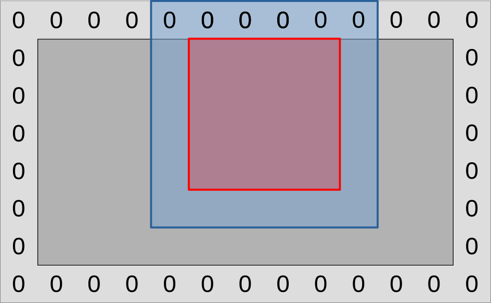
On the diagram above, a GPU workgroup now maps onto the entire colored region of the simulation domain, red and blue surfaces included.

As this workgroup begins to execute, each of its work-items will proceed to load the (U, V) data point associated with its current location from VRAM, then save it to a shared memory location that every other work-item in the workgroup has access to.

A workgroup barrier will then be used to wait for all work-items to be done. And after this, the work-items within the blue region will be done and exit the compute shader early. Meanwhile, work-items within the red region will proceed to load all their inputs from shared memory, then use these to compute the updated data point associated with their designated input location as before.

If we zoom out from this single workgroup view and try to get a picture of how the entire simulation domain maps into workgroups and work-items, it will look like this:

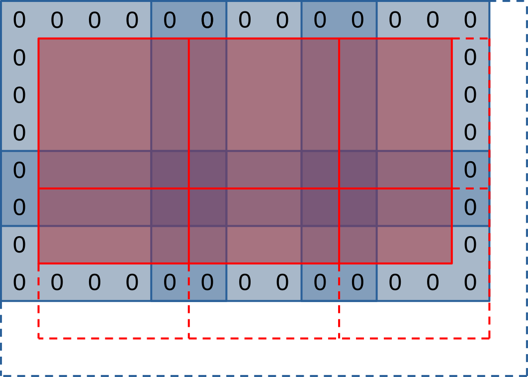
On the diagram above, each workgroup aims to produce a tile of outputs within the simulation domain (red square), and to this end it will first loading a larger set of input values (blue region) into shared memory. Much like in our initial algorithm, workgroups on the right and bottom edges of the simulation domain will extend beyond the end of it (dashed lines) and will need special care to avoid out-of-bounds memory reads and writes.

This picture lets you see that our new use of shared memory does not only come with advantages, but also has some drawbacks:

• The input regions of our work-groups (blue squares) overlap with each other (darker blue regions). This will result in some redundant input loads from VRAM.
• The outermost work-items of our work-groups exit early after loading simulation inputs. This will result in reduced execution efficiency as only a subset of each workgroup will participate in the rest of the computation.

Thankfully, this waste of memory and execution resource only concerns the outermost work-items of each work-group. Therefore, we expect that…

• Workgroups with a larger number of work-items should execute more efficiently, as they have more work-items in the central region and less in the edge region.
• Workgroups with a square-ish aspect ratio should execute more efficiently, as a square shape is mathematically optimal from the perspective of putting more work-items at the center of the workgroup and less on the edges.

But due to the conflicting constraints of GPU hardware (mapping of work-items to SIMD units, memory access granularity, maximal number of resources per workgroup, generation-dependent ability of NVidia hardware to reallocate idle work-items to other workgroups…), the reality is going to be more nuanced than “large square workgroups are better”, and we expect a certain hardware-specific workgroup size to be optimal. It it thus best to keep workgroup size as a tuning parameter that can be adjusted through empirical microbenchmarking, as we have done so far.

First implementation

Before we begin to use shared memory, we must first allocate it. The easiest and most performant way to do so, when available, is to allocate it at GLSL compile time. We can do this here by naming the specialization constants that control our workgroup size…

// In exercises/src/grayscott/common.comp

// This code looks stupid, but alas the rules of GLSL do not allow anything else
layout(local_size_x = 8, local_size_y = 8) in;
layout(local_size_x_id = 0, local_size_y_id = 1) in;
layout(constant_id = 0) const uint WORKGROUP_COLS = 8;
layout(constant_id = 1) const uint WORKGROUP_ROWS = 8;
const uvec2 WORKGROUP_SIZE = uvec2(WORKGROUP_COLS, WORKGROUP_ROWS);

…and allocating a matching amount of shared memory in which we will later store (U, V) values:

// In exercises/src/grayscott/step.comp

// Shared memory for exchanging (U, V) pairs between work-item
shared vec2 uv_cache[WORKGROUP_COLS][WORKGROUP_ROWS];

To make access to this shared memory convenient, we will then add a pair of functions. One lets a work-item store its (U, V) input at its designated location. The other lets a work item load data from shared memory at a certain relative offset with respect to its designated location.

// Save the (U, V) value that this work-item loaded so that the rest of the
// workgroup may later access it efficiently
void set_uv_cache(vec2 uv) {
   uv_cache[gl_LocalInvocationID.x][gl_LocalInvocationID.y] = uv;
}

// Get an (U, V) value that was previously saved by a neighboring work-item
// within this workgroup. Remember to use a barrier() first!
vec2 get_uv_cache(ivec2 offset) {
   const ivec2 shared_pos = ivec2(gl_LocalInvocationID.xy) + offset.xy;
   return uv_cache[shared_pos.x][shared_pos.y];
}

Now that this is done, we must rethink our mapping from GPU work-items to positions within the simulation domain, in order to acknowledge the fact that our work-groups overlap with each other. This concern will be taken care of by another new work_item_pos() GLSL function. And while we are at it, we will also add another is_workgroup_output() function, which tells if our work-item is responsible for producing an output data point.

// Size of the "border" at the edge of work-group, where work-items
// only read inputs and do not write outputs down
const uint BORDER_SIZE = 1;

// Size of the output region of a work-group, accounting for the input border
const uvec2 WORKGROUP_OUTPUT_SIZE = WORKGROUP_SIZE - 2 * uvec2(BORDER_SIZE);

// Truth that this work-item is within the output region of the workgroup
//
// Note that this is a necessary condition for emitting output data, but not a
// sufficient one. work_item_pos() must also fall inside of the output region
// of the simulation dataset, before data_end_pos().
bool is_workgroup_output() {
    const uvec2 OUTPUT_START = uvec2(BORDER_SIZE);
    const uvec2 OUTPUT_END = OUTPUT_START + WORKGROUP_OUTPUT_SIZE;
    const uvec2 item_id = gl_LocalInvocationID.xy;
    return all(greaterThanEqual(item_id, OUTPUT_START))
           && all(lessThan(item_id, OUTPUT_END));
}

// Position of the simulation dataset this work-item should read data from,
// and potentially write data to if it is in the central region of the workgroup
uvec2 work_item_pos() {
   const uvec2 workgroup_topleft = gl_WorkGroupID.xy * WORKGROUP_OUTPUT_SIZE;
   return workgroup_topleft + gl_LocalInvocationID.xy;
}

Given this, we are now ready to rewrite the beginning of our compute shader entry point, where inputs are loaded from VRAM. As before, we begin by finding out which position of our simulation domain our work-item maps into.

void main() {
   // Map work-items into a position within the simulation domain
   const uvec2 pos = work_item_pos();

   // [ ... ]

But after that, we are not allowed to immediately discard work-items which fall out of the simulation domain. Indeed, the barrier() GLSL function, which is used to wait until all work-items are done writing to shared memory, mandates that all work-items within the workgroup be still executing.

We must therefore keep around out of bounds work-items for now, using conditional logic to ensure that they do not perform out-of-bounds memory accesses.

// Load and share our designated (U, V) value, if any
vec2 uv = vec2(0.0);
if (all(lessThan(pos, padded_end_pos()))) {
    uv = read(pos);
    set_uv_cache(uv);
}

After this, we can wait for the workgroup to finish initializing its shared memory cache…

// Wait for the shared (U, V) cache to be ready
barrier();

…and it is only then that we will be able to discard out-of-bounds GPU work-items:

// Discard work-items that are out of bounds for output production work
if (!is_workgroup_output() || any(greaterThanEqual(pos, data_end_pos()))) {
    return;
}

Finally, we can adapt our diffusion gradient computation to use our new shared memory cache…

// Compute the diffusion gradient for U and V
const mat3 weights = stencil_weights();
vec2 full_uv = vec2(0.0);
for (int rel_y = -1; rel_y <= 1; ++rel_y) {
    for (int rel_x = -1; rel_x <= 1; ++rel_x) {
        const vec2 stencil_uv = get_uv_cache(ivec2(rel_x, rel_y));
        const float weight = weights[rel_x + 1][rel_y + 1];
        full_uv += weight * (stencil_uv - uv);
    }
}

…and the rest of the step compute shader GLSL code will not change.

The CPU side of the computation will not change much, but it does need two adjustments, one of the user input validation side and one of the simulation scheduling side.

Our new simulation logic, where workgroups have input-loading edges and an output production center, is incompatible with workgroups that contain less than 3 work-items on either side. We should therefore error out when the user requests such a work-group configuration, and we can do so by adding the following check at the beginning of the Pipelines::new() constructor:

// In exercises/src/grayscott/pipeline.rs

// Error out when an incompatible workgroup size is specified
let pipeline = &options.pipeline;
let check_side = |side: NonZeroU32| side.get() >= 3;
assert!(
    check_side(pipeline.workgroup_cols) && check_side(pipeline.workgroup_rows),
    "GPU workgroups must have at least three work-items in each dimension"
);

The schedule_simulation() function, which schedules the execution of the step compute pipeline, also needs to change, because our mapping from workgroups to simulation domain elements has changed. This is done by adjusting the initial simulate_workgroups computation to add a pair of - 2 that takes the input-loading edges out of the equation:

let dispatch_size = |domain_size: usize, workgroup_size: NonZeroU32| {
    domain_size.div_ceil(workgroup_size.get() as usize - 2) as u32
};
let simulate_workgroups = [
    dispatch_size(options.num_cols, options.pipeline.workgroup_cols),
    dispatch_size(options.num_rows, options.pipeline.workgroup_rows),
    1,
];

First benchmark

Unfortunately, this first implementation of the shared memory optimization does not perform as well as we would hope. Here is its effect on performance on the author’s AMD Radeon 5600M GPU:

run_simulation/workgroup8x8/domain2048x1024/total512/image32/compute
                        time:   [122.48 ms 122.61 ms 122.82 ms]
                        thrpt:  [8.7421 Gelem/s 8.7572 Gelem/s 8.7670 Gelem/s]
                 change:
                        time:   [-5.2863% -3.7811% -2.3117%] (p = 0.00 < 0.05)
                        thrpt:  [+2.3664% +3.9297% +5.5814%]
                        Performance has improved.

run_simulation/workgroup16x8/domain2048x1024/total512/image32/compute
                        time:   [124.89 ms 125.15 ms 125.41 ms]
                        thrpt:  [8.5621 Gelem/s 8.5795 Gelem/s 8.5978 Gelem/s]
                 change:
                        time:   [+21.130% +22.781% +24.736%] (p = 0.00 < 0.05)
                        thrpt:  [-19.831% -18.554% -17.444%]
                        Performance has regressed.

run_simulation/workgroup16x16/domain2048x1024/total512/image32/compute
                        time:   [197.14 ms 197.42 ms 197.68 ms]
                        thrpt:  [5.4318 Gelem/s 5.4388 Gelem/s 5.4466 Gelem/s]
                 change:
                        time:   [+76.474% +79.543% +82.293%] (p = 0.00 < 0.05)
                        thrpt:  [-45.143% -44.303% -43.334%]
                        Performance has regressed.

run_simulation/workgroup32x16/domain2048x1024/total512/image32/compute
                        time:   [192.35 ms 192.78 ms 193.23 ms]
                        thrpt:  [5.5567 Gelem/s 5.5696 Gelem/s 5.5824 Gelem/s]
                 change:
                        time:   [+105.24% +107.32% +109.64%] (p = 0.00 < 0.05)
                        thrpt:  [-52.300% -51.765% -51.277%]
                        Performance has regressed.

run_simulation/workgroup32x32/domain2048x1024/total512/image32/compute
                        time:   [222.67 ms 223.16 ms 223.40 ms]
                        thrpt:  [4.8063 Gelem/s 4.8116 Gelem/s 4.8221 Gelem/s]
                 change:
                        time:   [+124.76% +129.62% +135.86%] (p = 0.00 < 0.05)
                        thrpt:  [-57.602% -56.450% -55.508%]
                        Performance has regressed.

There are two things that are surprising about these results, and not in a good way:

1. We expected use of shared memory to improve our simulation’s performance, or at least not change it much if the GPU cache already knew how to handle the initial logic well. But instead our use of shared memory causes a major performance regression.
2. We expected execution and memory access inefficiencies related to the use of shared memory to have a lower impact on performance as the workgroup size gets larger. But instead the larger our workgroups are, the worse the performance regression gets.

Overall, it looks as if the more intensively we exercised shared memory with a larger workgroup, the more we ran into a severe hardware performance bottleneck related to our use of shared memory. Which begs the question: what could that hardware performance bottleneck be?

Bank conflicts

To answer this question, we need to look into how GPU caches, which shared memory is made of, are organized at the hardware level.

Like any piece of modern computing hardware, GPU caches are accessed via several independent load/store units that can operate in parallel. But sadly the circuitry associated with these load/store units is complex enough that hardware manufacturers cannot afford to provide one load/store unit per accessible memory location of the cache.

Instead of doing so, manufacturers therefore go for a compromise where some cache accesses can be processed in parallel and others must be serialized. Following an old hardware tradition, load/store units are organized such that memory accesses that target consecutive memory location are faster, and this is how we get the banked cache organization illustrated below:

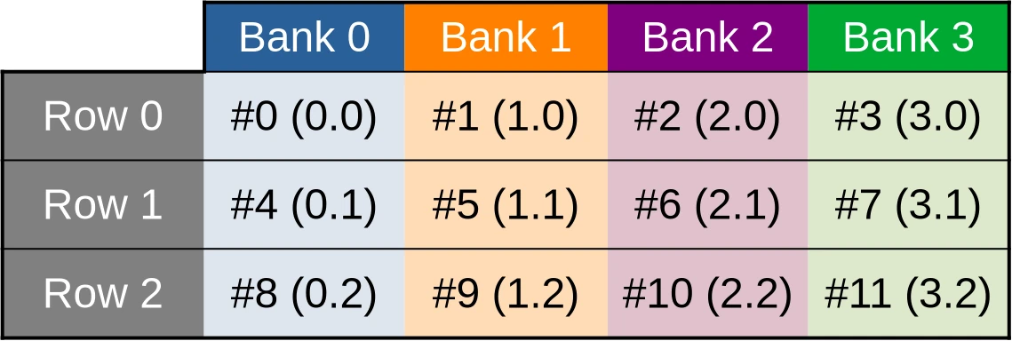
The toy cache example from this illustration possesses 4 independent storage banks (colored table columns), each of which controls 3 data storage cells (table rows). Memory addresses (denoted #N in the diagram) are then distributed across these storage cells in such a way that the first accessible address belongs to the first bank, the second location belongs to the second bank, and so on until we run out of banks. Then we start over at the first bank.

This storage layout ensures that if work is distributed across GPU work-items in such a way that the first work item processes the first shared memory location, the second work item processes the second shared memory location, and so on, then all cache banks will end up being evenly utilized, leading to maximal memory access parallelism and thus maximal performance.

However, things only work out so well as long as cached data are made of primitive 32-bit GPU data atoms. And as you may recall, this is not the case of our current shared memory cache, which is composed of two-dimensional vectors of such data:

// Shared memory for exchanging (U, V) pairs between work-item
shared vec2 uv_cache[WORKGROUP_COLS][WORKGROUP_ROWS];

Because of this, our (U, V) data cache ends up being organized in the following manner…

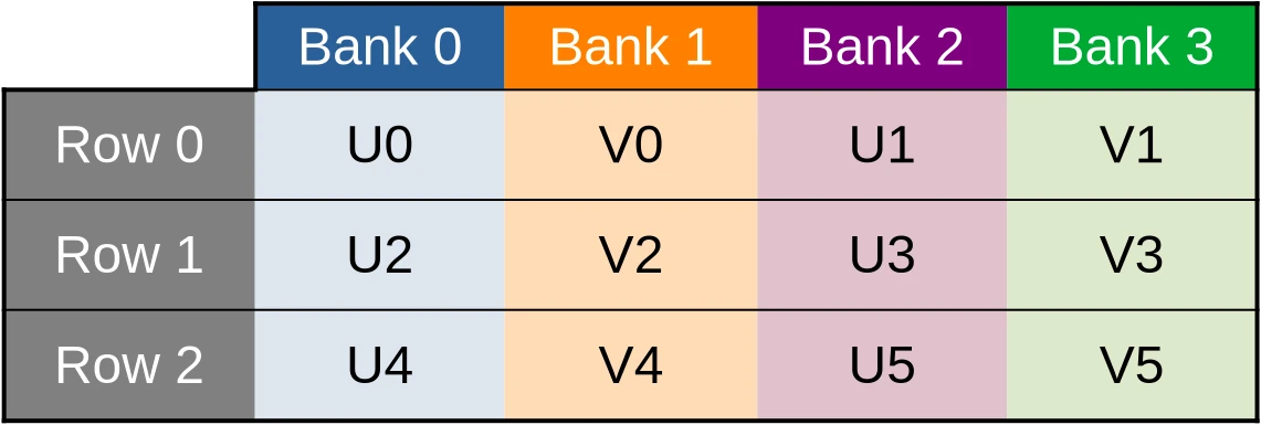
…which means that when the U component of the dataset is accessed via a first 32-bit memory load/store instruction, only one half of the cache banks end up being used…

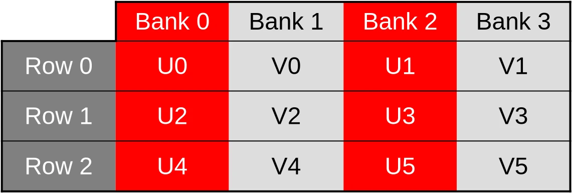
…and when the V component of the dataset later ends up being accessed by a second 32-bit memory load/store instruction, only the other half of the cache banks ends up being used.

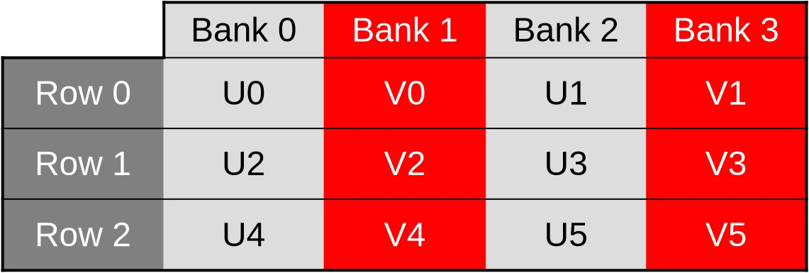
It gets worse than that, however. Our shared memory cache is also layed out as a two dimensional array where columns of data are contiguous in memory and rows of data are not.

This is a problem because in computer graphics, 2D images are conventionally layed out in memory such that rows of data are contiguous in memory, and columns are not. And because contiguous memory accesses are more efficient, GPUs normally optimize for this common case by distributing work-items over SIMD units in such a way that work-items on the same row (same Y coordinate, consecutive X coordinates) end up being allocated to the same SIMD unit and processed together.

In our shared memory cache, the data associated with those work-items ends up being stored inside of storage cells whose memory locations are separated by 2 * WORKGROUP_ROWS 32-bit elements. And when WORKGROUP_ROWS is large enough and a power of two, this number is likely to end up being a multiple of the number of cache memory data banks.

We will then end up with worst-case scenarios where cache bank parallelism is extremely under-utilized and all memory accesses from a given hardware SIMD instruction end up being sequentially processed by the same cache bank. For example, accesses to the U coordinate of the first row of data could be processed by the first cache bank…

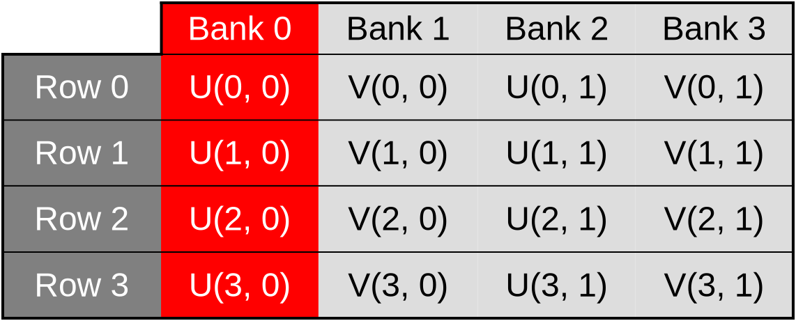
…accesses to the V coordinate of the first row could be processed by the second bank…

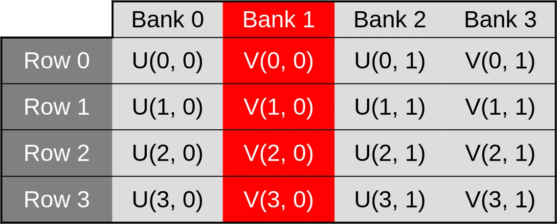
…accesses to the U coordinate of the second row could be processed by the third bank…

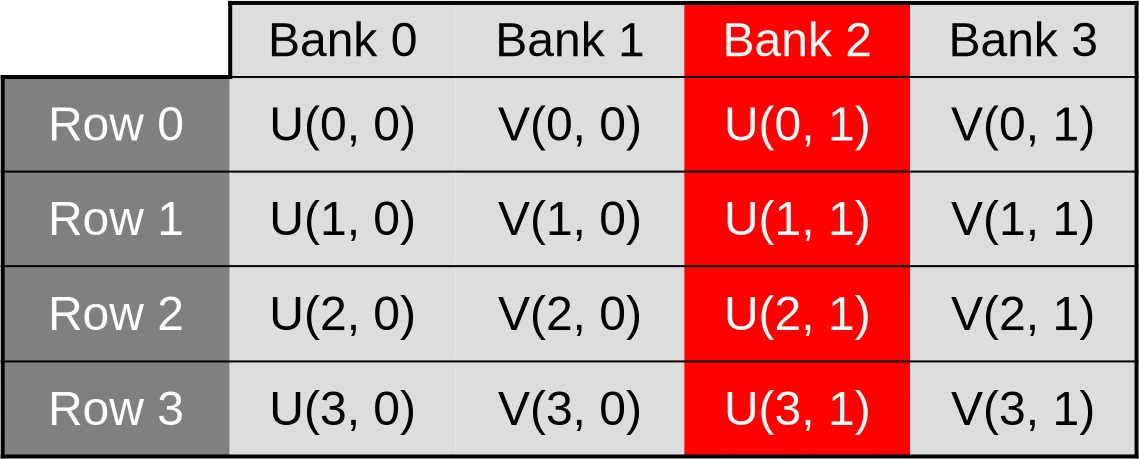
…and so on. This scenario, where cache bandwidth is under-utilized because memory accesses that could be processed in parallel are processed sequentially instead, is called a cache bank conflict.

Avoiding bank conflicts

While GPU cache bank conflicts can have a serious impact on runtime performance, they are thankfully easy to resolve once identified.

All we need to do here is to…

• Switch from our former “array-of-structs” data layout, where uv_cache is an array of two-dimensional vectors of data, to an alternate “struct-of-arrays” data layout where uv_cache begins with U concentration data and ends with V concentration data.
• Flip the 2D array axes so that work-items with consecutive X coordinates end up accessing shared memory locations with consecutive memory addresses.

In terms of code, it looks like this:

// Shared memory for exchanging (U, V) pairs between work-item
shared float uv_cache[2][WORKGROUP_ROWS][WORKGROUP_COLS];

// Save the (U, V) value that this work-item loaded so that the rest of the
// workgroup may later access it efficiently
void set_uv_cache(vec2 uv) {
   uv_cache[U][gl_LocalInvocationID.y][gl_LocalInvocationID.x] = uv.x;
   uv_cache[V][gl_LocalInvocationID.y][gl_LocalInvocationID.x] = uv.y;
}

// Get an (U, V) value that was previously saved by a neighboring work-item
// within this workgroup. Remember to use a barrier() first!
vec2 get_uv_cache(ivec2 offset) {
   const ivec2 shared_pos = ivec2(gl_LocalInvocationID.xy) + offset.xy;
   return vec2(
        uv_cache[U][shared_pos.y][shared_pos.x],
        uv_cache[V][shared_pos.y][shared_pos.x]
    );
}

After applying this simple data layout transform, our (U, V) data cache will end up being organized in the following manner…

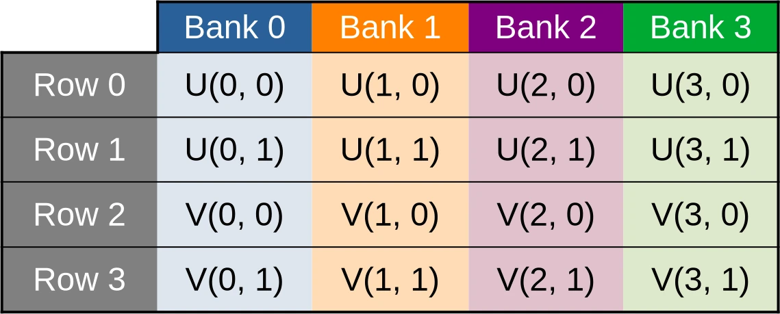
…where data points associated with the U species concentration for the first row of data are contiguous, and thus evenly spread across banks…

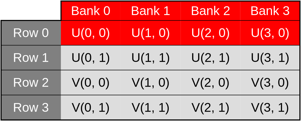
…and this remains true as we switch across rows, access the V species’ concentration, etc.

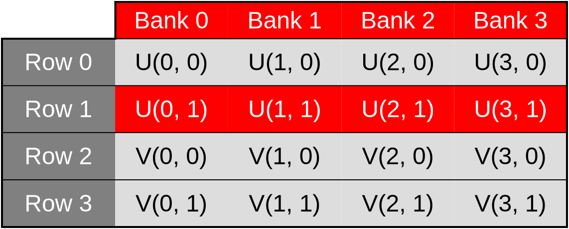
Because of this, we expect our new shared memory layout to result in a significant performance improvement, where individual shared memory accesses are sped up by up to 2x. Which will have a smaller, but hopefully still significant impact on the performance of the overall simulation.

Exercise

Implement this optimization and measure its performance impact on your hardware.

The improved shared memory layout that avoids bank conflicts should provide a net performance improvement over the original array-of-structs memory layout. But when comparing to the previous chapter, the performance tradeoff of manually managing a shared memory cache vs letting the GPU’s cache do this job is intrinsically hardware-dependent.

So don’t be disappointed if it turns out that on your GPU, using shared memory is not worthwhile even when cache bank conflicts are taken out of the equation.

Subgroups

On the author’s AMD Radeon 5600M GPU, avoiding shared memory bank conflicts is a major performance improvement. But not to the point where using shared memory ends up becoming an unambiguous step up in performance from the previous simulation implementation:

run_simulation/workgroup8x8/domain2048x1024/total512/image32/compute
                        time:   [119.78 ms 120.16 ms 120.56 ms]
                        thrpt:  [8.9060 Gelem/s 8.9356 Gelem/s 8.9641 Gelem/s]
                 change:
                        time:   [-7.0218% -5.5135% -4.0137%] (p = 0.00 < 0.05)
                        thrpt:  [+4.1815% +5.8352% +7.5521%]
                        Performance has improved.

run_simulation/workgroup16x8/domain2048x1024/total512/image32/compute
                        time:   [101.57 ms 101.85 ms 102.21 ms]
                        thrpt:  [10.505 Gelem/s 10.542 Gelem/s 10.571 Gelem/s]
                 change:
                        time:   [-1.6314% -0.1677% +1.4719%] (p = 0.85 > 0.05)
                        thrpt:  [-1.4505% +0.1680% +1.6584%]
                        No change in performance detected.

run_simulation/workgroup16x16/domain2048x1024/total512/image32/compute
                        time:   [100.44 ms 100.61 ms 100.82 ms]
                        thrpt:  [10.650 Gelem/s 10.672 Gelem/s 10.690 Gelem/s]
                 change:
                        time:   [-10.130% -8.5750% -7.1731%] (p = 0.00 < 0.05)
                        thrpt:  [+7.7274% +9.3793% +11.271%]
                        Performance has improved.

run_simulation/workgroup32x16/domain2048x1024/total512/image32/compute
                        time:   [96.656 ms 97.088 ms 97.459 ms]
                        thrpt:  [11.017 Gelem/s 11.059 Gelem/s 11.109 Gelem/s]
                 change:
                        time:   [+3.3377% +4.4153% +5.6007%] (p = 0.00 < 0.05)
                        thrpt:  [-5.3036% -4.2286% -3.2299%]
                        Performance has regressed.

run_simulation/workgroup32x32/domain2048x1024/total512/image32/compute
                        time:   [112.13 ms 112.37 ms 112.62 ms]
                        thrpt:  [9.5339 Gelem/s 9.5555 Gelem/s 9.5757 Gelem/s]
                 change:
                        time:   [+13.281% +15.723% +18.845%] (p = 0.00 < 0.05)
                        thrpt:  [-15.857% -13.587% -11.724%]
                        Performance has regressed.

It looks like for this particular GPU at least, either of the following is true:

1. The GPU’s cache handled our initial data access pattern very well, and thus manually managed shared memory is not a major improvement. And if it’s not an improvement, it can easily end up hurting due to the extra hardware instructions, barriers, etc.
2. We are still hitting some kind of hardware bottleneck related to our use of shared memory, that we could perhaps alleviate through further program optimization.

Unfortunately, to figure out what’s going on and get further optimization ideas if the second hypothesis is true, we need to use vendor profiling tools, and we will not be able to do so until a later chapter of this course. Therefore, it looks like we will be stuck with these somewhat disappointing shared memory performance for now.

What we can do, however, is experiment with a different Vulkan mechanism for exchanging data between work items, called subgroup operations. These operations are available on most (but not all) Vulkan-supported GPUs, and their implementation typically bypasses the cache entirely which allows them to perform faster than shared memory for some applications.

From architecture to API

For a long time, GPU APIs have focused on providing developers with the illusion that GPU programs execute over a large flat array of independent processing units, each having equal capabilities and an equal ability to communicate with other units.

However, this symmetric multiprocessing model is quite far from the reality of modern GPU hardware, which is implemented using a hierarchy of parallel execution and synchronization features. Indeed, since about 2010, GPU microarchitectures have standardized on many common decisions, and if you take a tour of any modern GPU you are likely to find…

• A variable amount of compute units¹ (from a couple to hundreds). Much like CPU cores, GPU compute units are mostly independent from each other, but do share some common resources like VRAM, last-level caches, and graphics-specific ASICs. These shared resources must be handled with care as they can easily become a performance bottleneck.
• Within each compute unit, there is a set of SIMD units² that share a fast cache. Each SIMD unit has limited superscalar execution capabilities, and most importantly can manage several concurrent instruction streams. The latter are used to improve SIMD ALU utilization in the face of high-latency operations like memory accesses: instead of waiting for the slow instruction from the current stream to complete, the SIMD unit switches to another instruction stream.³
• Within each concurrent SIMD instruction stream, we find instructions that, like all things SIMD, are designed to perform the same hardware operation over a certain amount of data points and to efficiently access memory in aligned and contiguous blocks. However GPU SIMD units have several features⁴ that make it easy to translate any combination of N parallel tasks into a sequence of SIMD instructions of width N, even when their behavior is far from regular SIMD logic, but at the expense of a performance degradation in such cases.

A naive flat parallelism model can be mapped onto such a hardware architecture by mapping each user-specified work-item to one SIMD lane within a SIMD unit and distributing the resulting SIMD instruction streams over the various compute units of the GPU. But by leveraging the specific features of each layer of this hierarchy, better GPU code performance can be achieved.

Sometimes this microarchitectural knowledge can be leveraged within the basic model given some knowledge/assumptions about how GPU drivers will map GPU API work to hardware. For example, seasoned GPU programmers know that work-items on a horizontal line (same Y and Z coordinates, consecutive X coordinates) are likely to be processed by the same SIMD unit, and should therefore be careful with divergent control flow and strive to access contiguous memory locations.

But there are microarchitectural GPU features that can only be leveraged if they are explicitly exposed in the API. For example, GPU compute shaders expose workgroups because these let programmers leverage some hardware features of GPU compute units:

• Hardware imposes API limits on how big workgroups can be and how much shared memory they can allocate, in order to ensures that a workgroup’s register and shared memory state can stay resident inside of a single GPU compute unit’s internal memory resources.
• Thanks to these restrictions, shared memory can be allocated out of the shared cache of the compute unit that all work-items in the workgroup have quick access to. And workgroup barriers can be efficiently implemented because 1/all associated communication stays local to a compute unit and 2/workgroup state is small enough to stay resident in a compute unit’s local memory resources while the barrier is being processed.

Subgroup operations are a much more recent addition to portable GPU APIs⁵ which aims to pick up where workgroups left off and expose capabilities of GPU SIMD units that can only be leveraged through explicit shader code changes. To give some examples of what subgroups can do, they expose the ability of many GPU SIMD units to…

• Tell if predication is currently being used, in order to let the GPU code take a fast path when operating in a pure SIMD execution regime.
• Perform an arithmetic reduction operation (sum, product, and/or/xor…) over the data points held by a SIMD vector. This is an important optimization when performing large-scale reductions, like computing the sum of all elements from an array, as it reduces the need for more expensive synchronization mechanisms like atomic operations.
• Efficiently transmit data between work-items that are processed by the same SIMD vector through shuffle operations. This is the operation that is most readily applicable to our diffusion gradient computation, and thus the one that we are agoing to explore in this chapter.

But of course, since this is GPU programming, everything cannot be so nice and easy…

Issues & workarounds

Hardware/driver support

Subgroups did not make the cut for the Vulkan 1.0 release. Instead, they were gradually added as optional extensions to Vulkan 1.0, then later merged into Vulkan 1.1 core in a slightly different form. This raises the question: should Vulkan code interested in subgroups solely focus on the Vulkan 1.1 version of the feature, or also support the original Vulkan 1.0 extensions?

To answer this sort of questions, we can use the https://vulkan.gpuinfo.org database, where GPU vendors and individuals regularly upload the Vulkan support status of a particular (hardware, driver) combination. The data has various known issues, for example it does not reflect device market share (all devices have equal weight), and the web UI groups devices by driver-reported name (which varies across OSes and driver versions). But it is good enough to get a rough idea of how widely supported/exotic a particular Vulkan version/extension/optional feature is.

If we ignore reports older than 2 years (which reduces the device name change issue), we reach the conclusion that of 3171 reported device names, only 57 (1.8%) do not support Vulkan 1.1 as of their latest driver version. From this, we can conclude that Vulkan 1.0 extensions are probably not worth supporting, and we should focus on the subgroup support that was added to Vulkan 1.1 only.

That is not the end of it, however, because Vulkan 1.1 only mandates very minimal subgroup support out of Vulkan implementations, which is insufficient for our needs:

• Subgroups only need to be supported in of compute shaders. That’s good enough for us.
• Subgroups of size 1 are allowed, as a way to support hardware without driver-exposed SIMD instructions. But those are useless for our data exchange purposes, so we will not be able to use subgroup shuffle operations on such implementations.
• The only nontrivial subgroup operation that Vulkan 1.1 mandates support for is the election of a “leader” work-item. This is not enough for our purposes, we need shuffle operations too.

Therefore, before we can use subgroups, we should probe the following physical device properties:

• Vulkan 1.1 should be supported, as we will use Vulkan 1.1 subgroup operations.
• Relative⁶ shuffle operations should be supported, enabling fast data exchanges.
• Subgroups should have ≥ 3 elements (minimum for left/right neighbor exchanges⁷).

Finally, there is one last thing to take care of when it comes to hardware/driver specifics. On many GPUs, subgroup size is not a fixed hardware-imposed parameter as Vulkan 1.1 device properties would have you believe. It is rather a user-tunable parameter that can be configured at various power-of-two sizes between two bounds. For example, AMD GPUs support subgroup sizes of 32 and 64, while Apple Mx GPUs support subgroup sizes of 4, 8, 16 and 32.

Being able to adjust the subgroup size like this is useful because there is an underlying performance tradeoff. Roughly speaking…

• Larger subgroups tend to perform better in ideal conditions (homogeneous conditional logic, aligned and contiguous memory accesses, few barriers, abundant concurrency). But smaller subgroups tend to be more resilient to less ideal conditions.
• On hardware where large subgroups are implemented through multi-cycle execution over narrower SIMD ALUs, like current AMD GPUs, shuffle operations may perform better at smaller subgroup sizes that match the true hardware SIMD unit width.

Subgroup size control was historically exposed via the VK_EXT_subgroup_size_control extension to Vulkan 1.1, which was integrated into Vulkan 1.3 core as an optional feature. But a quick GPUinfo query suggests that at the time of writing, there are many more devices/drivers that support the extension than devices/drivers that support Vulkan 1.3 core. Therefore, as of 2025, it is a good idea to support both ways of setting the subgroup size.

Absence of this functionality is not a dealbreaker, but when it is there, it is good practice to benchmark at all available subgroup sizes in order to see which one works best.

Undefined 2D layout

We have been using 2D workgroups with a square-ish aspect ratio so far because they map well into our 2D simulation domain and guarantee some degree of hardware cache locality.

However, there is a problem with such workgroups when subgroups get involved, which is that Vulkan does not specify how 2D workgroups will be decomposed into 1D subgroups. In other words, all of the ways of decomposing a 4x4 workgroup into 4-element subgroups that are illustrated below are valid in the eyes of the Vulkan 1.1 specification:

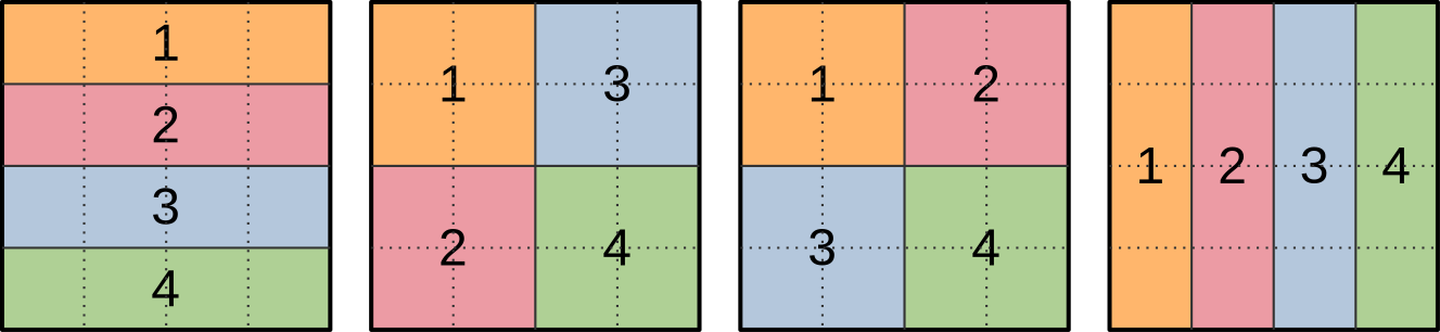
This would not be an issue if we were using subgroup operations for data reduction, where the precise order in which input data points are aggregated into a final result generally does not matter. But it is an issue for our intended use of subgroup shuffles, which is to exchange input concentration data with neighboring work-items.

Indeed, if we don’t know the spatial layout of subgroups, then we cannot know ahead of time whether, say, the previous work-item in the subgroup lies at our left, on top, or someplace else in the simulation domain that may not be a nearest neighbor at all.

We could address this by probing the subgroup layout at runtime. But given that we are effectively trying to optimize the overhead of a pair of memory loads, the computational overhead of such a runtime layout check is quite unlikely to be acceptable.

We will therefore go for the less elegant alternative of exclusively using one-dimensional workgroups that lie over a horizontal line, as there is only one logical decomposition of these into subgroups…

…and thus we know that when performing relative subgroup shuffles, the previous work-item (if any) will be our left neighbor, and the next work-item (if any) will be our right neighbor.

Speaking of which, there is another matter that we need to take care of before we start using relative subgroup shuffles. Namely figuring out a sensible way to handle the first work-item in a subgroup (which has no left neighbor within the subgroup) and the last work-item in a subgroup (which has no right neighbor within the subgroup).

Undefined shuffle outputs

As mentioned before, our end goal here is to use relative subgroup shuffles operations. These effectively shift data forward or backward within the subgroup by N places, as illustrated below…

…but as the ? character on the illustration illustrates, there is a problem at the edges of the subgroup, where we are effectively pulling data out of non-existent subgroup work-items before the first one and after the last one.

The Vulkan specification declares that these data values are undefined, and we certainly do not want to use them in our computation. Instead, we basically have two sane options:

1. We use subgroups in the standard way by making each element of the subgroup produce one output data point, but the first and last work-item in the subgroup do not follow the same logic as other work-items and pull their left/right input value from memory.
2. As we did with work-groups back in the shared memory chapter, we make subgroups process overlapping regions of the simulation domain, such that the first/last work-item of each subgroup only participates in input data loading and exits early after the shuffles instead of participating in the rest of the computation.

The first option may sound seducive, as it allows all work-items within the subgroups to participate in the final simulation computation. But it does not actually work well on GPU hardware, especially when applied within a single subgroup, because subgroups are implemented using SIMD. Which means that if the work-items at the edge of a subgroup do something slow, other work-items in the subgroup will end up waiting for them and become equally slow as a result.

Therefore, we will take the second option: even though the spatial distribution of subgroups within our grid of work-items looks like this from the GPU API’s perspective…

…we will actually decompose each subgroup such that its edge elements only participate in input loading and shuffling, leaving the rest of the simulation work to central elements only:

And then we will make the input region of subgroups overlap with each other, so that their output regions end up being contiguous, as with our previous 2D workgroup layout for shared memory:

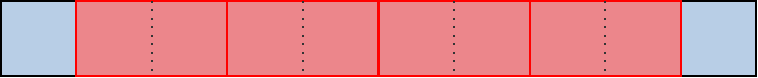
At this point, you may reasonably wonder whether this is actually a performance improvement. After all, on the above illustrations, we turned subgroups that produced 4 data points into subgroups that only produce 2 data points by removing one element on each edge, and thus lost ~half or our computing resources during a large fraction of the simulation computation!

But the above schematics were made for clarity, not realism. A quick trip to the GPUinfo database will tell you that in the real world, ~96% of Vulkan implementations that are true GPUs (not CPU emulations thereof) use a subgroup size of 32 or more, with 32 being by far the most common case.

Given subgroups of 32 work-items, reserving two work-items on the edges for input loading tasks only sacrifices <10% of available computing throughput…

…and thus a visual representation of two 32-elements subgroups that overlap with each other, while less readable and amenable to detailed explanations, certainly looks a lot less concerning:

Knowing this, we will hazard the guess that if using subgroups offers a significant speedup over loading data from VRAM and the GPU cache hierarchy (which remains to be proven), it will likely be worth the loss of two work items per subgroup on most common hardware.

And if benchmarking on less common configurations with small subgroups later reveals that this subgroup usage pattern does not work for them, as we suspect, then we will be able to handle this by simply bumping the hardware requirements of our subgroup-based algorithms, so that they are only used when sufficiently large subgroups are available.

Ill-defined reconvergence

Finally, there is one last subgroup gotcha that will not be a very big problem for us, but spells trouble for enough other subgroup-based algorithms that it is worth discussing here.

Consider the following GLSL conditional execution pattern:

void main() {

  // Entire workgroup is active here

  if (sg_condition) {

    // Some subgroups are inactive here, others are fully active
    // i.e. sg_condition has the same value for all work-items of each subgroup

    if (item_condition_1) {

      // Some work-items of a subgroup are masked out by item_condition_1 here
      // i.e. item_condition is _not_ homogeneous across some subgroups

      if (item_condition_2) {

        // More work-items are masked out by item_condition_2 here
        // i.e. item_condition_2 is _not_ homogeneous even across those
        // work-items for which item_condition_1 is true.

      }

      // Now let's call this code location #1...

    }

    // ...this code location #2...

  }

  // ...and this code location #3

}

As this compute shader executes, subgroups within a compute workgroup will reach the first condition sg_condition. Subgroups for which this condition is false will skip over this if statement and move directly to code location #3.

So far, this is not a very concerning situation, because SIMD units remain fully utilized without predication masking out lanes. The only situation where such conditional branching could possibly be a problem is if sg_condition is only true for a few sugroups, which can lead to compute units becoming under-utilized as most subgroups exit early while the remaining one keep blocking the GPU from moving on to the next (dependent) compute dispatch.

But after this first conditional statement, subgroups for which sg_condition is true reach the item_condition_1 condition, which can only be handled through SIMD predication. And then…

• SIMD unit utilization efficiency decreases because while the SIMD lanes for which item_condition_1 is true keep working, the remaining SIMD lanes remain idle, waiting for the end of the if (item_condition_1) block to be reached before resuming execution.
• Some subgroup operations like relative shuffles start behaving weirdly because they operate on data from SIMD lanes that have been masked out, resulting in undefined results. Generally speaking, subgroup operations must be used with care in this situation.

In the GPU world, this scenario is called divergent execution, and it is a very common source of performance problems. But as you can see, in the presence of subgroup operations, it can become a correctness problem too.

In any case, after this execution proceeds and we reach item_condition_2, which makes the problem worse, but does not fundamentally change the situation. But the most interesting question is what happens next, at the end of the if statements?

Many GPU programmers new to subgroups naively expect that as soon as an if statement ends, the subgroup will immediately get back to its state before the if statement started, with previously disabled work-items re-enabled, as illustrated below…

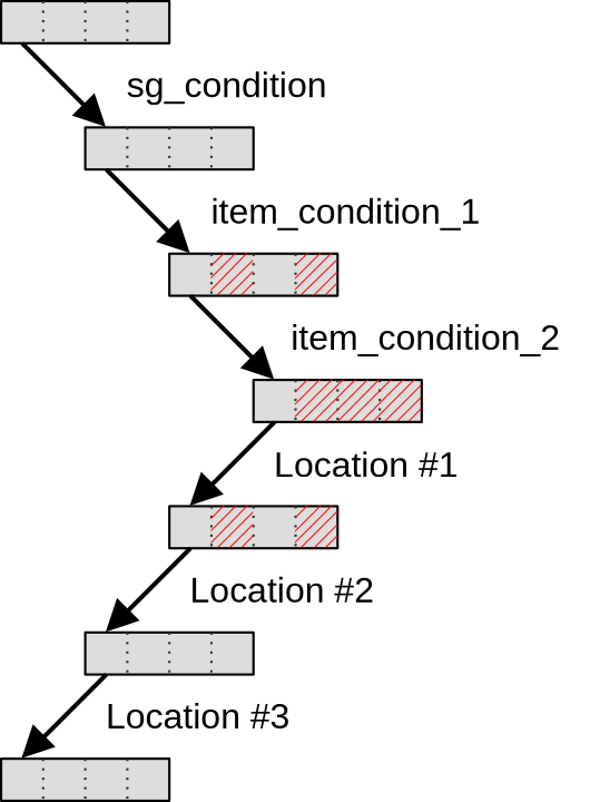
…but the Vulkan 1.1 specification does not actually guarantee this and allows implementations to keep subgroups in a divergent state until the end of the first if statement that was taken by the entire workgroup. Which in our case is program location #3, after the end of the initial if (sg_subgroup) statement.

Until this point of the program is reached, Vulkan implementations are free to keep executing statements multiple times with divergent control flow if they so desire, as illustrated below:

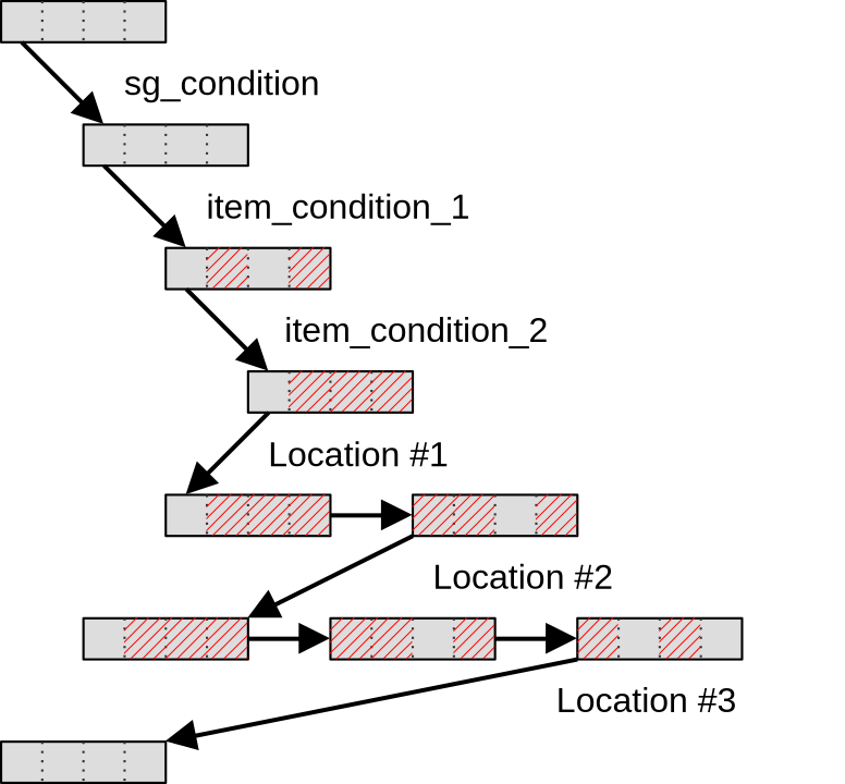
The reason why Khronos decided to allow this behavior in Vulkan 1.1 is not fully clear. Perhaps there are devices on which switching subgroups between a predicated and non-predicated state is expensive, in which case the above scheme could be more efficient in situations where there is little code at locations #1 and #2? But in any case, this implementor freedom makes usage of subgroup operations inside of conditional statements more fraught with peril than it should be.

In an attempt to reduce this peril, several Vulkan extensions were therefore proposed, each exposing a path towards saner subgroup reconvergence behavior on hardware that supports it.

At first, in 2020, the VK_KHR_shader_subgroup_uniform_control_flow extension was introduced. This extension guarantees that if conditional statements in the GLSL code are manually annotated as being uniform across entire subgroups, then subgroup control flow will be guaranteed to reconverge no later than at the end of the first control flow statement that was not subgroup-uniform. In other words, when using this extension with suitable code annotations, we have a guarantee that subgroups will reconverge at code location #2 as illustrated below:

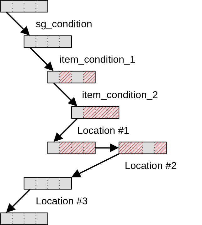
For some subgroup-based algorithms, however, that guarantee is still not enough, which is why in 2021 a stricter VK_KHR_shader_maximal_reconvergence extension was released. This new extension guarantees that if it is enabled, and entire SPIR-V shader modules are annotated with a suitable attribute, then within these shader modules subgroups will reconverge as much as possible at the end of each conditional statement, getting us back to the programmer intuition we started with:

However, as of 2025, these two Vulkan extensions are quite far from having universal hardware & driver support, and therefore all Vulkan code that aims for broad hardware portability should only use them as a fast path while still providing a fallback code path that is very careful about using subgroup operations inside of conditional statements.

And in doing so, one should also keep in mind that although the above explanation was given in terms of nested if statements, the same principles hold for any kind of control flow divergence across a subgroup, including switch statements with a value that varies across work-items, for loops with a number of iteration that varies across work items, and a ? b : c ternary operators.

Thankfully, as you will see later in this chapter, this particular Vulkan specification issue will not affect our Gray-Scott reaction simulation much, because it has little conditional logic in it and the one that we do have will not do too much harm. It is only mentioned in this course as an important subgroup gotcha that you should be aware of when you will consider using Vulkan subgroup operations in more complex GPU computations.

First implementation: 1D workgroups

Mapping GPU work-items to data

To make the migration towards subgroups easier, we will start with a simple mapping of the dataset to GPU workgroups. First of all, we will cut the output region of the simulation domain into lines that are one data point tall…

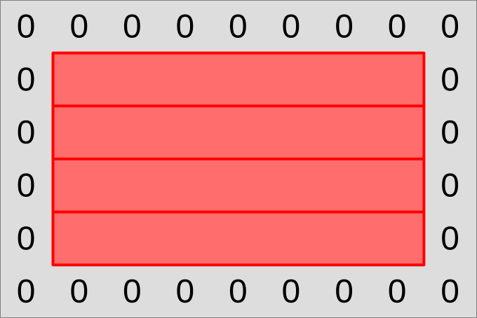
…and have each output line be processed by a workgroup that also has a line shape:

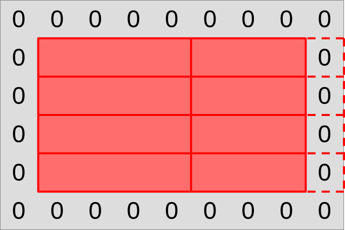
These 1D workgroups will then be further subdivided by the GPU into 1D subgroups, that we will each make responsible for producing one chunk of the workgroup output.

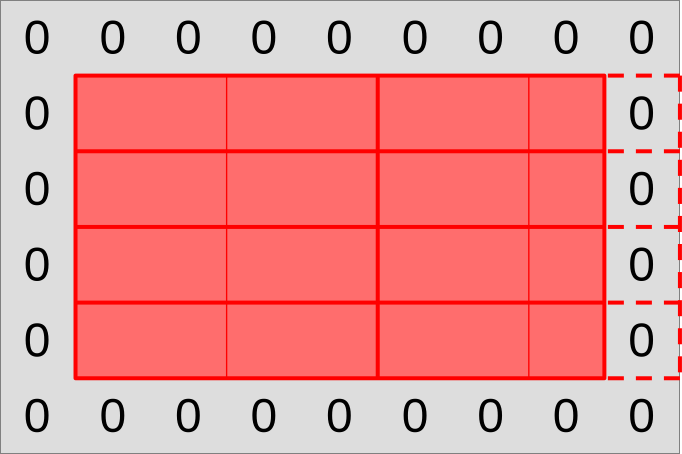
However, we will not follow the naive chunking of workgroups into subgroups that the GPU’s standard work-item grid hints us into. As explained earlier, our subgroups will overlap with each other, as the input region of each subgroup will extend one data point left and right into the output region of the neighboring subgroup. This will let us get our left and right neighbor value through relative shuffles, without conditional memory loads that would ruin our SIMD efficiency.

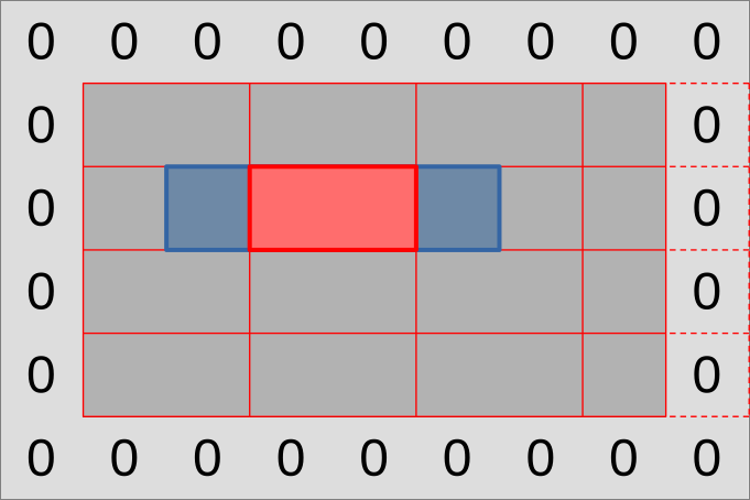
As in previous simulation implementations, we will need to be careful with subgroups that reside on the edge of the simulation domain:

• The rightmost work-items may reside beyond the edges of the simulation domain and should not load input data from the (U, V) input dataset.
• If this happens, the work-item that plays the role of the right input neighbor and is only used for data loading may not be the last work-item of the subgroup.
• With larger workgroups, we may even get entire subgroups that extend outside of the simulation domain. We will have to make those exit early without using them at all.

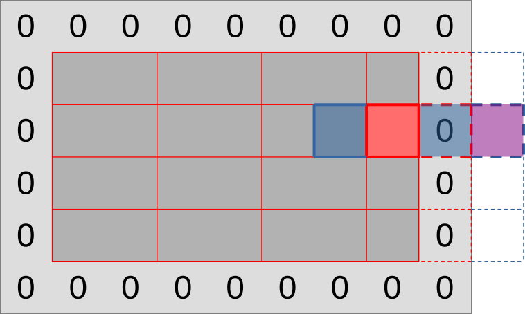
Finally, our diffusion gradient computation will need top and bottom data points, which we can get through a variation of the same strategy:

• Load a whole line of inputs above/below the output region using the entire subgroup. This will give each work-item that produces an output value its top/bottom neighbor value
• Use relative shuffle operations to get topleft/topright values from the neighboring top value, and bottomleft/bottomright neighbor values from the neighboring bottom value.

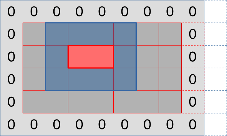
Overall, the full picture will look like the illustration below: rows of output that are hierarchically subdivided into workgroups then subgroups, with supporting memory loads around the edge and some out-of-bounds work-items to take care of on the right edge (but not on the bottom edge).

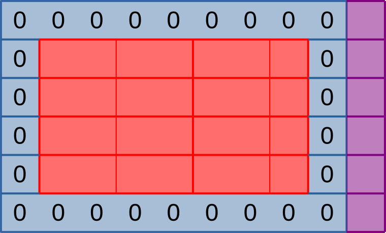
Forcing the use of 1D workgroups

To implement the above scheme, we must first modify our simulation so that it only allows the use of 1D workgroups. This can be done in three steps:

• Revert changes from the shared memory chapter. This 1D workgroup layout is incompatible with our current shared memory scheme, which requires workgroups to have at least three rows. Later in this chapter, we will see how to use shared memory again without needing 2D workgroups of undefined subgroup layout.
• Remove the workgroup_rows field of the PipelineOptions struct, replacing each use in the code of with the literal integer 1 or removing it as appropriate. While we are at it, consider also renaming the workgroup_cols field to workgroup_sizeand adjusting each use in the code as appropriate, this will come in handy later on.
• Rework the top-level loop of the simulate benchmark so that instead of instead of iterating over [workgroup_cols, workgroup_rows] pairs, it iterates over one-dimensional work-group sizes of [64, 128, 256, 512, 1024]. You will also need to adjust the benchmark group name format string to "run_simulation/workgroup{workgroup_size}/domain{num_cols}x{num_rows}/total{total_steps}".

After this is done, consider doing doing a microbenchmark run to see how switching to 1D workgroups affected benchmark performance. If your GPU is like the author’s Radeon 5600M, you should observe that when going from 2D square-ish workgroups to 1D workgroups with the same number of work-items, the performance impact ranges from neutral to positive.

The fact that on this particular GPU/driver combination, 2D workgroups are not actually helpful to performance, in spite of having better theoretical cache locality properties, suggests that AMD GPUs happens to schedule workgroups in such a way that good cache locality is achieved anyway.⁸ But we will later see how to guarantee good cache locality without relying on lucky scheduling like this.

On the solution branch, we also performed a GPU pipeline refactor to remove the now-unused WORKGROUP_ROWS GLSL specialization constant, rename WORKGROUP_COLS to WORKGROUP_SIZE, and shift specialization constant IDs by one place to make them contiguous again…

// Configurable workgroup size, as before
layout(local_size_x = 64, local_size_y = 1) in;
layout(local_size_x_id = 0) in;
layout(constant_id = 0) const uint WORKGROUP_SIZE = 64;

// Concentration table width
layout(constant_id = 1) const uint UV_WIDTH = 1920;

// "Scalar" simulation parameters
layout(constant_id = 2) const float FEED_RATE = 0.014;
layout(constant_id = 3) const float KILL_RATE = 0.054;
layout(constant_id = 4) const float DELTA_T = 1.0;

// [ ... subtract 1 from all other constant_id, adapt host code ... ]

…but that’s a bit annoying for only a slight improvement in code readability, so do not feel forced to do it. If you don’t do it, the only bad consequence is that you will need to replace future occurences of WORKGROUP_SIZE in the code samples with the old WORKGROUP_COLS name.

New compute pipeline

Subgroup operations are not part of the core GLSL specification, they are part of the GL_KHR_shader_subgroup extension. To be more precise, we are going to need the GL_KHR_shader_subgroup_shuffle_relative GLSL extension, which itself is defined by the GL_KHR_shader_subgroup GLSL extension specification.

We can check can check if the GLSL extension is supported by our GLSL compiler using a GLSL preprocessor define with the same name, and if so enable it using the #extension directive…

#ifdef GL_KHR_shader_subgroup_shuffle_relative
  #extension GL_KHR_shader_subgroup_shuffle_relative : require
#endif

…but unfortunately, such checking is not very useful in a Vulkan world, as it only checks for extension support within our GLSL compiler. This compiler is only used at application build time to generate a SPIR-V binary that the device driver will later consume at runtime, and it is the feature support of this device that we are actually interested in, but cannot probe from the GLSL side.

In principle, we could work around this by keeping two versions of our compute shader around, one that uses subgroups that doesn’t, but given that…

• Vulkan 1.1 is supported by 98.2% of devices whose Vulkan support was reported to GPUinfo in the past 2 years. Of those, 99.3% support relative shuffle operations and 98.9% have a subgroup size of 4 or more that is compatible with our minimal requirements.
• Juggling between two versions of a shader depending on which features a Vulkan device supports, where one shader version will almost never be exercised and is thus likely to bitrot over future software maintenance, feels excessive for a pedagogical example.

…we will bite the bullet and unconditionally require relative subgroup shuffle support.

// To be added to exercises/src/grayscott/step.comp, after #version

#extension GL_KHR_shader_subgroup_shuffle_relative : require

However, in the interest of correctness, we will later check on the host that the device meets our requirements, and abort the simulation if it doesn’t.

In any case, as in the shared memory chapter, we will need some logic to check whether our work-item is tasked with producing an output data point, and if so where that data point is located within the simulation domain. The mathematical formula changes, but the idea remains the same.

// To be added to exercises/src/grayscott/tep.comp, after #include

// Number of input-only work-items on each side of a subgroup
const uint BORDER_SIZE = 1;

// Maximal number of output data points per subgroup
//
// Subgroups on the edge of the simulation domain may end up processing fewer
// data points.
uint subgroup_output_size() {
    return gl_SubgroupSize - 2 * BORDER_SIZE;
}

// Truth that this work-item is within the output region of the subgroup
//
// Note that this is a necessary condition for emitting output data, but not a
// sufficient one. work_item_pos() must also fall inside of the output region
// of the simulation dataset, before data_end_pos().
bool is_subgroup_output() {
    return (gl_SubgroupInvocationID >= BORDER_SIZE)
           && (gl_SubgroupInvocationID < BORDER_SIZE + subgroup_output_size());
}

// Maximal number of output data points per workgroup (see above)
uint workgroup_output_size() {
    return gl_NumSubgroups * subgroup_output_size();
}

// Position of the simulation dataset that corresponds to the central value
// that this work-item will eventually write data to, if it ends up writing
uvec2 work_item_pos() {
    const uint first_x = DATA_START_POS.x - BORDER_SIZE;
    const uint item_x = gl_WorkGroupID.x * workgroup_output_size()
                        + gl_SubgroupID * subgroup_output_size()
                        + gl_SubgroupInvocationID
                        + first_x;
    const uint item_y = gl_WorkGroupID.y + DATA_START_POS.y;
    return uvec2(item_x, item_y);
}

What is new to this chapter, however, is that we will now also have a pair of utility functions that let us shuffle (U, V) data pairs from one work-item of the subgroup to another, using the only relative shuffle patterns that we care about in this simulation:

// To be added to exercises/src/grayscott/step.comp, between above code & main()

// Data from the work-item on the right in the current subgroup
//
// If there is no work-item on the right, or if it is inactive, the result will
// be an undefined value.
vec2 shuffle_from_right(vec2 data) {
    return vec2(
        subgroupShuffleDown(data.x, 1),
        subgroupShuffleDown(data.y, 1)
    );
}

// Data from the work-item on the left in the current subgroup
//
// If there is no work-item on the left, or if it is inactive, the result will
// be an undefined value.
vec2 shuffle_from_left(vec2 data) {
    return vec2(
        subgroupShuffleUp(data.x, 1),
        subgroupShuffleUp(data.y, 1)
    );
}

After this, our simulation shader entry point will, as usual, begin by assigning a spatial location to the active work-item and loading the associated data value.

Since we have stopped using shared memory for now, we can make work-items that cannot load data from their assigned location exit early.

void main() {
    // Map work items into 2D dataset, discard those outside input region
    // (including padding region).
    const uvec2 pos = work_item_pos();
    if (any(greaterThanEqual(pos, padded_end_pos()))) {
        return;
    }

    // Load central value
    const vec2 uv = read(pos);

    // [ ... rest of the shader follows ... ]

After this, we will begin the diffusion gradient computation, iterating over lines of input as usual.

But instead of iterating over columns immediately after that, we will proceed to set up storage for a full line of three inputs (left neighbor, central value, and right neighbor), and load the central value at our work item’s assigned horizontal position.

    // Compute the diffusion gradient for U and V
    const uvec2 top = pos - uvec2(0, 1);
    const mat3 weights = stencil_weights();
    vec2 full_uv = vec2(0.0);
    for (int y = 0; y < 3; ++y) {
        // Read the top/center/bottom value
        vec2 stencil_uvs[3];
        stencil_uvs[1] = read(top + uvec2(0, y));

        // [ ... rest of the diffusion gradient computation follows ... ]

The left and right neighbor values will then be obtained via shuffle operations. As the comment above these operations highlights, these shuffles will return invalid values for some work-items, but that’s fine because these work-items will not produce outputs. They are only used for the purpose of loading and shffling inputs.

        // Get the left/right value from neighboring work-items
        //
        // This will be garbage data for the work-items on the left/right edge
        // of the subgroup, but that's okay, we'll filter these out with an
        // is_subgroup_output() condition later on.
        //
        // It can also be garbage on the right edge of the simulation domain
        // where the right neighbor has been rendered inactive by the
        // padded_end_pos() filter above, but if we have no right neighbor we
        // are only loading data from the zero edge of the simulation dataset,
        // not producing an output. So our garbage result will be masked out by
        // the other pos < data_end_pos() condition later on.
        stencil_uvs[0] = shuffle_from_left(stencil_uvs[1]);
        stencil_uvs[2] = shuffle_from_right(stencil_uvs[1]);

        // [ ... rest of the diffusion gradient computation follows ... ]

The diffusion gradient computation will then proceed as usual for the current line of inputs, and the whole cycle will repeat for our three lines of input…

        // Add associated contributions to the stencil
        for (int x = 0; x < 3; ++x) {
            full_uv += weights[x][y] * (stencil_uvs[x] - uv);
        }
    }

    // [ ... rest of the computation follows ... ]

…at which point we will be done with the diffusion gradient computation.

After this computation, we know won’t need the left/right work-items from the subgroup anymore (which computed garbage from undefined shuffle outputs anyway), so we can dispose of them.

    // Discard work items that are out of bounds for output production work, or
    // that received garbage at the previous shuffling stage.
    if (!is_subgroup_output() || any(greaterThanEqual(pos, data_end_pos()))) {
        return;
    }

    // [ ... rest of the computation is unchanged ... ]

And beyond that, the rest of the simulation shader will not change.

If you try to compile the simulation program at this stage, you will notice that our shaderc GLSL-to-SPIRV compiler is unhappy because we are using subgroup operations, which require a newer SPIR-V version than what vulkano requires by default.

It is okay to change this in pipeline.rs, in doing so we are not bumping our device requirements further than we already did by deciding to mandate Vulkan 1.1 earlier:

// To be changed in exercises/src/grayscott/pipeline.rs

/// Shader modules used for the compute pipelines
mod shader {
    vulkano_shaders::shader! {
        spirv_version: "1.3",  // <- This is new
        shaders: {
            init: {
                ty: "compute",
                path: "src/grayscott/init.comp"
            },
            step: {
                ty: "compute",
                path: "src/grayscott/step.comp"
            },
        }
    }
}

New device requirements

By going the lazy route of mandating subgroup shuffle support, we gained a few device support requirements. We will therefore encode them into a utility function at the root of the grayscott code module…

// To be added to exercises/src/grayscott/mod.rs

use vulkano::{
  device::physical::{PhysicalDevice, SubgroupFeatures},
  Version,
};

/// Check that the selected Vulkan device meets our requirements
pub fn is_suitable_device(device: &PhysicalDevice) -> bool {
    let properties = device.properties();
    device.api_version() >= Version::V1_1
        && matches!(
            properties.subgroup_supported_operations,
            Some(ops) if ops.contains(SubgroupFeatures::SHUFFLE_RELATIVE)
        )
        && matches!(
            properties.subgroup_size,
            Some(size) if size >= 3
        )
}

…check that these requirements are met at the beginning of run_simulation()…

// To be changed in exercises/src/grayscott/mod.rs

/// Simulation runner, with a user-specified output processing function
pub fn run_simulation<ProcessV: FnMut(ArrayView2<Float>) -> Result<()>>(
    options: &RunnerOptions,
    context: &Context,
    process_v: Option<ProcessV>,
) -> Result<()> {
    // Check that the selected Vulkan device meets our requirements
    assert!(
        is_suitable_device(context.device.physical_device()),
        "Selected Vulkan device does not meet the Gray-Scott simulation requirements"
    );

    // [ ... rest of the function is unchanged ... ]
}

…and modify the Vulkan context’s default device selection logic (when the user does not explicitly pick a Vulkan device) to select a device that meets those requirements:

// To be changed in exercises/src/context.rs

/// Pick a physical device
fn select_physical_device(
    instance: &Arc<Instance>,
    options: &DeviceOptions,
    quiet: bool,
) -> Result<Arc<PhysicalDevice>> {
    let mut devices = instance.enumerate_physical_devices()?;
    if let Some(index) = options.device_index {
        // [ ... user-specified device code path is unchanged ... ]
    } else {
        // Otherwise, choose a device according to its device type
        devices
            // This filter() iterator adaptor is new
            .filter(|dev| crate::grayscott::is_suitable_device(dev))
            .min_by_key(|dev| match dev.properties().device_type {
                // [ ... device ordering is unchanged ... ]
            })
            .inspect(|device| {
                // [ ... and logging is unchanged ... ]
            })
            .ok_or_else(|| "no Vulkan device available".into())
    }
}

Dispatch configuration changes

Finally, we need to adjust the number of work-groups that are spawned in order to match our new launch configuration. So we adjust the start of the schedule_simulation() function to compute the new number of workgroups on the X axis…

// To be changed in exercises/src/grayscott/mod.rs

/// Record the commands needed to run a bunch of simulation iterations
fn schedule_simulation(
    options: &RunnerOptions,
    context: &Context,  // <- Need to add this parameter
    pipelines: &Pipelines,
    concentrations: &mut Concentrations,
    cmdbuild: &mut CommandBufferBuilder,
) -> Result<()> {
    // Determine the appropriate dispatch size for the simulation
    let subgroup_size = context
        .device
        .physical_device()
        .properties()
        .subgroup_size
        .expect("Should have checked for subgroup supports before we got here");
    let subgroup_output_size = subgroup_size - 2;
    let subgroups_per_workgroup = options
        .pipeline
        .workgroup_size
        .get()
        .checked_div(subgroup_size)
        .expect("Workgroup size should be a multiple of the subgroup size");
    let outputs_per_workgroup = subgroups_per_workgroup * subgroup_output_size;
    let workgroups_per_row = options.num_cols.div_ceil(outputs_per_workgroup as usize) as u32;
    let simulate_workgroups = [workgroups_per_row, options.num_rows as u32, 1];

    // [ ... rest of the simulation scheduling is unchanged ... ]
}

…and this means that schedule_simulation() now needs to have access to the Vulkan context, so we pass that new parameter too in the caller of schedule_simulation(), which is SimulationRunner::schedule_next_output():

// To be changed in exercises/src/grayscott/mod.rs

impl<'run_simulation, ProcessV> SimulationRunner<'run_simulation, ProcessV>
where
    ProcessV: FnMut(ArrayView2<Float>) -> Result<()>,
{
    // [ ... constructor is unchanged ... ]

    /// Submit a GPU job that will produce the next simulation output
    fn schedule_next_output(&mut self) -> Result<FenceSignalFuture<impl GpuFuture + 'static>> {
        // Schedule a number of simulation steps
        schedule_simulation(
            self.options,
            self.context,  // <- This parameter is new
            &self.pipelines,
            &mut self.concentrations,
            &mut self.compute_cmdbuild,
        )?;

        // [ ... rest is unchanged ... ]

Notice that we have introduced a new condition that the workgroup size be a multiple of the subgroup size. That’s because Vulkan normally allows workgroup sizes not to be a multiple of the subgroup size, by starting one or more subgroups in a state where some SIMD lanes are disabled (in the case of our 1D workgroup, it will be the last lanes). But we don’t want to allow it because…

1. It’s inefficient, since the affected subgroup(s) don’t execute at full SIMD throughput.
2. It’s hard to support, in our case we would need to replace our simple is_subgroup_output() GLSL logic with a more complicated one that checks whether we are in the last workgroup and if so adjusts our expectations about what the last subgroup lane should be.

In any case, however well-intentioned, this change is affecting the semantics of a user-visible interface for subgroup size tuning, so we should…

• Document that the workgroup size should be a multiple of the subgroup size in the CLI help text about PipelineOptions::workgroup_size.
• Adjust the default value of this CLI parameter so that it is guaranteed to always be a multiple of the device’s subgroup size. Since the maximal subgroup size supported by Vulkan is 128, and Vulkan subgroup sizes are guaranteed to be a power of two this means that our default workgroup size should be at least 128, or a multiple thereof.

Overall, the updated PipelineOptions definition looks like this…

// Change in exercises/src/grayscott/pipeline.rs

/// CLI parameters that guide pipeline creation
#[derive(Debug, Args)]
pub struct PipelineOptions {
    /// Number of work-items in a workgroup
    ///
    /// Must be a multiple of the Vulkan device's subgroup size.
    #[arg(short = 'W', long, default_value = "128")]
    pub workgroup_size: NonZeroU32,

    // [ ... rest is unchanged ... ]
}

…and you should also remove the microbenchmark configuration for workgroup sizes of 64, which has never performed well anyway.

With that, we are ready to run our first subgroups-enabled simulation. But we still are at the mercy of the device-selected subgroup size for now, which may not be the one that works best for our algorithm. Let’s see how we can fix that next.

Using subgroup size control

As mentioned earlier, subgroup size control was first specified as a VK_EXT_subgroup_size_control extension to Vulkan 1.1, and later integrated into the core Vulkan 1.3 specification. However, at the time of writing, the vulkano Rust bindings that we are using only support the Vulkan 1.3 version of this specification. We will therefore only support subgroup size control for Vulkan 1.3 devices.

There are two key parts to using Vulkan 1.3 subgroup size control:

• Because it is an optional device feature, we must first enable it at the time where a logical Device is created, via the enabled_features field of the DeviceCreateInfo struct.
  • As this is a Vulkan 1.3 specific feature, and Vulkan 1.3 is far from being universally supported at the time of writing, we will not want to force this feature on. It should either be enabled by explicit user request, or opportunistically when the device supports it.
• Given a Vulkan device for which subgroup size control has been enabled, the subgroup size of a compute pipeline can then be set at construction time by setting the required_subgroup_size field of the associated PipelineShaderStageCreateInfo. In doing so, we must respect the rules outlined in the documentation of required_subgroup_size:
  • The user-specified subgroup size must be a power of two ranging between the min_subgroup_size and max_subgroup_size device limits. These device limits were added to the device properties by Vulkan 1.3, which from a vulkano perspective means that the associated optional fields of DeviceProperties will always be set on Vulkan 1.3 compliant devices.
  • Compute pipeline workgroups must not contain more subgroups than dictated by the Vulkan 1.3 max_compute_workgroup_subgroups device limit. This new limit supplements the max_compute_work_group_invocations limit that had been present since Vulkan 1.0 by acknowledging the fact that one some devices, the maximum work group size is specified as a number of subgroups, and is thus subgroup size dependent.

Enabling device support + context building API refactor

Having to enable a device feature first is a bit of an annoyance in the exercises codebase layout, because it means that our new subgroup size setting (which is a parameter of compute pipeline building in the Gray-Scott simulation) will end up affecting device building (which is handled by our Vulkan context building code, which we’ve been trying to keep quite generic so far).

And this in turn means that we will once again need to add a parameter to the Context::new() constructor and adapt all of its clients, including our old square program that does not use subgroup size control. Clearly, this is not great API design, so let’s give our Context constructor a quick round of API redesign that reduces the need for such client adaptations in the future.

All of the Context constructor parameters that we have been adding over time represent optional Vulkan context features that have an obvious default setting:

• The quiet parameter inhibits logging for microbenchmarks. Outside of microbenchmarks, logging should always be enabled, so that is a fine default setting.
• The progress parameter makes logging interoperate nicely with the indicatif progress bars, which are only used by the simulate binary. Outside of the simulate binary and other future programs with indicatif progress bar, there is no need to accomodate indicatif’s constraints and we should log to stderr directly.

As you’ve seen before in the vulkano API, a common way to handle this sort of “parameters with obvious defaults” in Rust is to pack them into a struct with a default value…

/// `Context` configuration that is decided by the code that constructs the
/// context, rather than by the user (via environment or CLI)
#[derive(Clone, Default)]
pub struct ContextAppConfig {
    /// When set to true, this boolean flag silences all warnings
    pub quiet: bool,

    /// When this is configured with an `indicatif::ProgressBar`, any logging
    /// from `Context` will be printed in an `indicatif`-aware manner pub
    progress: Option<ProgressBar>,

    // [ ... subgroup size control enablement coming up ... ]
}

…then make it a parameter to the function of interest and later, on the client side, override only the parameters of interest and use the default value for all other fields:

// Example of ContextAppConfig configuration from a microbenchmark
ContextAppConfig {
    quiet: true,
    ..Default::default()
}

The advantage of doing this this way is that as we later add support for new context features, like subgroup size control, existing clients will not need to be changed as long as they do not need the new feature. And in this way, API backwards compatibility will be achieved.

In our case, we know ahead of time that we are going to want an extra parameter to control subgroup size control, so let’s do it right away:

// Add to exercises/src/context.rs

/// `Context` configuration that is decided by the code that constructs the
/// context, rather than by the user (via environment or CLI)
#[derive(Clone, Default)]
pub struct ContextAppConfig {
    /// When set to true, this boolean flag silences all warnings
    pub quiet: bool,

    /// When this is configured with an `indicatif::ProgressBar`, any logging
    /// from `Context` will be printed in an `indicatif`-aware manner
    pub progress: Option<ProgressBar>,

    /// Truth that the Vulkan 1.3 `subgroupSizeControl` feature should be
    /// enabled (requires Vulkan 1.3 device with support for this feature)
    pub subgroup_size_control: SubgroupSizeControlConfig,
}

/// Truth that the `subgroupSizeControl` Vulkan extension should be enabled
#[derive(Copy, Clone, Default, Eq, PartialEq)]
pub enum SubgroupSizeControlConfig {
    /// Do not enable subgroup size control
    ///
    /// This is the default and requires no particular support from the device.
    /// But it prevents `subgroupSizeControl` from being used.
    #[default]
    Disable,

    /// Enable subgroup size control if supported
    ///
    /// Code that uses this configuration must be prepared to receive a device
    /// that may or may not support subgroup size control.
    IfSupported,

    /// Always enable subgroup size control
    ///
    /// Device configuration will fail if the user requests a device that does
    /// not support subgroup size control, or if autoconfiguration does not find
    /// a device that supports it.
    Enable,
}

As you can see, we are going to want to support three subgroup size control configurations:

• Do not enable subgroup size control. This is the default, and it suits old clients that don’t use subgroup size control like the square computation very well.
• Enable subgroup size control if it is supported, otherwise ignore it. This configuration is perfect for microbenchmarks, which want to exercise multiple subgroup sizes if available, without dropping support for devices that do not support Vulkan 1.3.
• Unconditionally enable subgroup size control. This is the right thing to do if the user requested that a specific subgroup size be used.

We will then refactor our Context::new() constructor to use the new ContextAppConfig struct instead of raw parameters, breaking its API one last time, and adjust downstream functions to pass down this struct or individual members thereof as appropriate.

// To be changed in exercises/src/context.rs

impl Context {
    /// Set up a `Context`
    pub fn new(options: &ContextOptions, app_config: ContextAppConfig) -> Result<Self> {
        let library = VulkanLibrary::new()?;
        let mut logging_instance =
            LoggingInstance::new(library, &options.instance, app_config.progress.clone())?;
        let physical_device =
            select_physical_device(&logging_instance.instance, &options.device, &app_config)?;
        let DeviceAndQueues {
            device,
            compute_queue,
            transfer_queue,
        } = DeviceAndQueues::new(physical_device, &app_config)?;
        // [ ... rest of context building does not change ... ]
    }
}

This means that select_physical_device() now takes a full app_config instead of a single quiet boolean parameter:

/// Pick a physical device
fn select_physical_device(
    instance: &Arc<Instance>,
    options: &DeviceOptions,
    app_config: &ContextAppConfig,
) -> Result<Arc<PhysicalDevice>> {
    // [ ... change all occurences of `quiet` to `app_config.quiet` here ... ]
}

And there is a good reason for this, which is that if the user explicitly required subgroup size control with SubgroupSizeControlConfig::Enable, our automatic device selection logic within this function must adapt. Otherwise, we could accidentally select a device that does not support subgroup size control even if there’s another device on the machine that does, resulting in an automatic device configuration that errors out when it could not do so.

We handle that by having around a new function that tells if a Vulkan device supports subgroup size control for compute shaders…

// Add to exercises/src/context.rs

use vulkano::{shader::ShaderStages, Version};

/// Check for compute shader subgroup size control support
pub fn supports_compute_subgroup_size_control(device: &PhysicalDevice) -> bool {
    if device.api_version() < Version::V1_3 {
        return false;
    }
    if !device.supported_features().subgroup_size_control {
        return false;
    }
    device
        .properties()
        .required_subgroup_size_stages
        .expect("Checked for Vulkan 1.3 support above")
        .contains(ShaderStages::COMPUTE)
}

…and adding this check to our device filter within select_physical_device(), which formerly only checked that subgroup support was good enough for our Gray-Scott simulation:

// Change in exercises/src/context.rs

/// Pick a physical device
fn select_physical_device(
    instance: &Arc<Instance>,
    options: &DeviceOptions,
    app_config: &ContextAppConfig,
) -> Result<Arc<PhysicalDevice>> {
    let mut devices = instance.enumerate_physical_devices()?;
    if let Some(index) = options.device_index {
        // [ ... known-device logic is unchanged ... ]
    } else {
        // Otherwise, choose a device according to its device type
        devices
            .filter(|dev| {
                if !crate::grayscott::is_suitable_device(dev) {
                    return false;
                }
                if app_config.subgroup_size_control == SubgroupSizeControlConfig::Enable
                    && !supports_compute_subgroup_size_control(dev)
                {
                    return false;
                }
                true
            })
            // [ ... rest of the iterator pipeline is unchanged ... ]
    }
}

Finally, we make DevicesAndQueues::new() enable subgroup size control as directed…

impl DeviceAndQueues {
    /// Set up a device and associated queues
    fn new(device: Arc<PhysicalDevice>, app_config: &ContextAppConfig) -> Result<Self> {
        // [ ... queue selection is unchanged ... ]

        // Decide if the subgroupSizeControl Vulkan feature should be enabled
        let subgroup_size_control = match app_config.subgroup_size_control {
            SubgroupSizeControlConfig::Disable => false,
            SubgroupSizeControlConfig::IfSupported => {
                supports_compute_subgroup_size_control(&device)
            }
            SubgroupSizeControlConfig::Enable => true,
        };
        let enabled_features = DeviceFeatures {
            subgroup_size_control,
            ..Default::default()
        };

        // Set up the device and queues
        let (device, mut queues) = Device::new(
            device,
            DeviceCreateInfo {
                queue_create_infos,
                enabled_features,
                ..Default::default()
            },
        )?;

        // [ ... rest is unchanged ... ]
    }
}

…and as far as the context-building code is concerned, we are all set.

Finally, we switch the square binary and microbenchmark to the new Context::new() API for what will hopefully be the last time.

// Change in exercises/src/bin/square.rs

use grayscott_exercises::context::ContextAppConfig;

fn main() -> Result<()> {
    // Parse command line options
    let options = Options::parse();

    // Set up a Vulkan context
    let context = Context::new(&options.context, ContextAppConfig::default())?;

    // [ ... rest is unchanged ... ]
}


// Change in exercises/benches/square.rs

use grayscott_exercises::context::ContextAppConfig;

// Benchmark for various problem sizes
fn criterion_benchmark(c: &mut Criterion) {
    // Iterate over device numbers, stopping on the first failure (which we
    // take as evidence that no such device exists)
    for device_index in 0.. {
        let context_options = ContextOptions {
            instance: InstanceOptions { verbose: 0 },
            device: DeviceOptions {
                device_index: Some(device_index),
            },
        };
        let app_config = ContextAppConfig {
            quiet: true,
            ..Default::default()
        };
        let Ok(context) = Context::new(&context_options, app_config.clone()) else {
            break;
        };

        // Benchmark context building
        let device_name = &context.device.physical_device().properties().device_name;
        c.bench_function(&format!("{device_name:?}/Context::new"), |b| {
            b.iter(|| {
                Context::new(&context_options, app_config.clone()).unwrap();
            })
        });

        // [ ... rest is unchanged ... ]
    }
}

Let’s not adapt the Gray-Scott binary and benchmark to this API yet, though. We have other things to do on that side before we can set that new subgroup_size_control parameter correctly.

Simulation subgroup size control

In the Gray-Scott simulation’s pipeline module, we will begin by adding a new optional simulation CLI parameter for explicit subgroup size control, which can also be set via environment variables for microbenchmarking convenience. This is just a matter of adding a new field to the PipelineOptions struct with the right annotations:

// Change in exercises/src/grayscott/pipeline.rs

/// CLI parameters that guide pipeline creation
#[derive(Debug, Args)]
pub struct PipelineOptions {
    /// Number of work-items in a workgroup
    #[arg(short = 'W', long, default_value = "64")]
    pub workgroup_size: NonZeroU32,

    /// Enforce a certain number of work-items in a subgroup
    ///
    /// This configuration is optional and may only be set on Vulkan devices
    /// that support the Vulkan 1.3 `subgroupSizeControl` feature.
    #[arg(env, short = 'S', long)]
    pub subgroup_size: Option<NonZeroU32>,

    // [ ... rest is unchanged ... ]
}

We will then adjust our compute stage setup code so that it propagates this configuration to our compute pipelines when it is present…

/// Set up a compute stage from a previously specialized shader module
fn setup_compute_stage(
    module: Arc<SpecializedShaderModule>,
    options: &PipelineOptions,  // <- Need this new parameter
) -> PipelineShaderStageCreateInfo {
    let entry_point = module
        .single_entry_point()
        .expect("a compute shader module should have a single entry point");
    PipelineShaderStageCreateInfo {
        required_subgroup_size: options.subgroup_size.map(NonZeroU32::get),
        ..PipelineShaderStageCreateInfo::new(entry_point)
    }
}

…which means the pipeline options must be passed down to setup_compute_stage() now, so the Pipelines::new() constructor needs a small adjustment:

impl Pipelines {
    pub fn new(options: &RunnerOptions, context: &Context) -> Result<Self> {
        fn setup_stage_info(
            options: &RunnerOptions,
            context: &Context,
            load: impl FnOnce(
                Arc<Device>,
            )
                -> std::result::Result<Arc<ShaderModule>, Validated<VulkanError>>,
        ) -> Result<PipelineShaderStageCreateInfo> {
            // [ ... beginning is unchanged ... ]
            Ok(setup_compute_stage(module, &options.pipeline))
        }

        // [ ... rest is unchanged ... ]
    }
}

We must then adjust the simulation scheduling code so that it accounts for the subgroup size that is actually being used, which is not necessarily the default subgroup size from Vulkan 1.1 device properties anymore…

// Change in exercises/src/grayscott/mod.rs

/// Record the commands needed to run a bunch of simulation iterations
fn schedule_simulation(
    options: &RunnerOptions,
    context: &Context,
    pipelines: &Pipelines,
    concentrations: &mut Concentrations,
    cmdbuild: &mut CommandBufferBuilder,
) -> Result<()> {
    // Determine the appropriate dispatch size for the simulation
    let subgroup_size = if let Some(subgroup_size) = options.pipeline.subgroup_size {
        subgroup_size.get()
    } else {
        context
            .device
            .physical_device()
            .properties()
            .subgroup_size
            .expect("Should have checked for subgroup supports before we got here")
    };
    // [ ... rest is unchanged ... ]
}

…and we must adjust the main simulation binary so that during the Vulkan context setup stage, it requests support for subgroup size control if the user has asked for it via the compute pipeline options. We will obviously also migrate it to the new ContextAppConfig API along the way:

// Change in exercises/src/bin/simulate.rs

use grayscott_exercises::context::ContextAppConfig;

fn main() -> Result<()> {
    // [ ... beginning is unchanged ... ]

    // Set up the Vulkan context
    let context = Context::new(
        &options.context,
        ContextAppConfig {
            progress: Some(progress.clone()),
            subgroup_size_control: if options.runner.pipeline.subgroup_size.is_some() {
                SubgroupSizeControlConfig::Enable
            } else {
                SubgroupSizeControlConfig::Disable
            },
            ..Default::default()
        },
    )?;

    // [ ... rest is unchanged ... ]
}

Microbenchmarking at all subgroup sizes

Finally, let us migrate our simulation microbenchmark to use subgroup size control. Here, the behavior that we want is a bit more complex than for the main simulation binary:

• By default, we want to benchmark at all available subgroup sizes if subgroup size control is available. If it is not available, on the other hand, we only benchmark at the default Vulkan 1.1 subgroup size as we did before. This lets us explore the full capabilities of newer devices without increasing our minimal device requirements on the other end.
• Probing all subgroup sizes increases benchmark duration by a multiplicative factor, which can be very large on some devices (there are embedded GPUs out there that support all subgroup sizes from 4 to 128). Therefore, once the optimal subgroup size has been determined, we let the user benchmark at this subgroup size only via the SUBGROUP_SIZE environment variable (which controls the subgroup_size field of our PipelineOptions through clap magic). Obviously, in that case, we will need to force subgroup size control on, as in any other case where the user specifies the desired subgroup size control.

This behavior can be implemented in a few steps. First of all, we adjust the Vulkan context setup code so that subgroup size control is always enabled if the user specified an explicit subgroup size, and enabled if supported otherwise. Along the way, we migrate our Vulkan context setup to the new ContextAppConfig API:

// Change in exercises/benches/simulate.rs

use grayscott_exercises::context::{
    ContextAppConfig,
    SubgroupSizeControlConfig,
};

fn criterion_benchmark(c: &mut Criterion) {
    // Start from the default context and runner options
    let context_options = default_args::<ContextOptions>();
    let mut runner_options = default_args::<RunnerOptions>();

    // Set up the Vulkan context
    let context = Context::new(
        &context_options,
        ContextAppConfig {
            quiet: true,
            subgroup_size_control: if runner_options.pipeline.subgroup_size.is_some() {
                SubgroupSizeControlConfig::Enable
            } else {
                SubgroupSizeControlConfig::IfSupported
            },
            ..Default::default()
        },
    )
    .unwrap();

    // [ ... other changes coming up next ... ]
}

We then set up a Vec of optional explicit subgroup sizes to be benchmarked:

• If subgroup size control is not supported, then there is a single None entry, which models the default subgroup size from Vulkan 1.1.
• Otherwise there is one Some(size) entry per subgroup size that should be exercised.

That approach is admittedly not very elegant, but it will make it easier to support presence or absence of subgroup size control with a single code path later on.

We populate this table according to the logic discussed above: user-specified subgroup size takes priority, then subgroup size control if supported, otherwise default subgroup size.

    use grayscott_exercises::context;

    // [ ... after Vulkan context setup ... ]

    // Determine which subgroup size configurations will be benchmarked
    //
    // - If the user specified a subgroup size via the SUBGROUP_SIZE environment
    //   variable, then we will only try this one.
    // - Otherwise, if the device supports subgroup size control, then we will
    //   try all supported subgroup sizes.
    // - Finally, if the device does not support subgroup size control, we have
    //   no choice but to use the default subgroup size only.
    let mut subgroup_sizes = Vec::new();
    if runner_options.pipeline.subgroup_size.is_some() {
        subgroup_sizes.push(runner_options.pipeline.subgroup_size);
    } else if context::supports_compute_subgroup_size_control(context.device.physical_device()) {
        let device_properties = context.device.physical_device().properties();
        let mut subgroup_size = device_properties.min_subgroup_size.unwrap();
        let max_subgroup_size = device_properties.max_subgroup_size.unwrap();
        while subgroup_size <= max_subgroup_size {
            subgroup_sizes.push(Some(NonZeroU32::new(subgroup_size).unwrap()));
            subgroup_size *= 2;
        }
    } else {
        subgroup_sizes.push(None);
    }

    // [ ... more to come ... ]

Within the following loop ove workgroup sizes, we then inject a new loop over benchmarked subgroup sizes. When an explicit subgroup size is specified, our former device support test is extended to also take the new max_compute_workgroup_subgroups limit into account. And if the selected subgroup size is accepted, we inject into the PipelineOptions used by the benchmark.

    // [ ... after subgroup size enumeration ... ]

    // For each workgroup size of interest...
    for workgroup_size in [64, 128, 256, 512, 1024] {
        // ...and for each subgroup size of interest...
        for subgroup_size in subgroup_sizes.iter().copied() {
            // Check if the device supports this workgroup configuration
            let device_properties = context.device.physical_device().properties();
            if workgroup_size > device_properties.max_compute_work_group_size[0]
                || workgroup_size > device_properties.max_compute_work_group_invocations
            {
                continue;
            }
            if let Some(subgroup_size) = subgroup_size
                && workgroup_size.div_ceil(subgroup_size.get())
                    > device_properties.max_compute_workgroup_subgroups.unwrap()
            {
                continue;
            }

            // Set up the pipeline
            runner_options.pipeline = PipelineOptions {
                workgroup_size: NonZeroU32::new(workgroup_size).unwrap(),
                subgroup_size,
                update: runner_options.pipeline.update,
            };

            // [ ... more to come ... ]
        }
    }
}

Finally, when we configure our criterion benchmark group, we indicate any explicitly configured subgroup size in the benchmark name so that benchmarks with different subgroup sizes can be differentiated from each other and filtered via a regex.

                    // [ ... at the top of the loop over total_steps ... ]

                    // Benchmark groups model a certain total amount of work
                    let mut group_name = format!("run_simulation/workgroup{workgroup_size}");
                    if let Some(subgroup_size) = subgroup_size {
                        write!(group_name, "/subgroup{subgroup_size}").unwrap();
                    }
                    write!(
                        group_name,
                        "/domain{num_cols}x{num_rows}/total{total_steps}"
                    )
                    .unwrap();
                    let mut group = c.benchmark_group(group_name);
                    group.throughput(Throughput::Elements(
                        (num_rows * num_cols * total_steps) as u64,
                    ));
                    
                    // [ ... rest is unchanged ... ]

And that’s it. We are now ready to benchmark our subgroups-enabled simulation at all subgroup sizes supported by our GPU.

First benchmark results

TODO: Check output in wave32 mode and benchmark wrt async-download-1d.

Guaranteeing 2D cache locality

As hinted above, our initial mapping of GPU work-items to data was intended to be easier to understand and make introduction of subgroup operations easier, but it has several flaws:

• From a memory bandwidth savings perspective, subgroup operations give us good reuse of every input data points across left/right neighbors. But our long line-like 1D workgroups do not guarantee much reuse of input datapoints across top/bottom neighbors, hampering cache locality. We may get some cache locality back if the GPU work scheduler happens to schedule workgroups with the same X position and consecutive Y positions on the same compute unit, but that’s just being lucky as nothing in the Vulkan spec guarantees this behavior.
• From an execution efficiency perspective, workgroups that extend far across one spatial direction are not great either, because it is likely that on the right edge they will extend far beyond the end of the simulation domain, and this will reduce in lots of wasted scheduling work (Vulkan device will spawn lots of subgroups/work-items that cannot even load input data and must exit immediately).

Due of these two issues, it would be better for our work-items to cover a simulation domain region that extends over the two dimensions of space, in a shape that gets as close to square as possible.

But as we have seen before, we cannot simply do so by using workgroups that have a 2D shape within the GPU-defined work grid, because when we do that our subgroup spatial layout becomes undefined and we cannot efficiently tell at compile time which work-item within the subgroup is a left/right neighbor of the active work-item anymore.

However, there is a less intuitive way to get where we want, which is to ask for 1D work-groups from the GPU API, but then map them over a 2D spatial region by having each subgroup process a different line of the simulation domain at the GLSL level.

In other words, instead of spatially laying out the subgroups of a workgroup in such a way that their output region forms a contiguous line, as we did before…

…we will now stack their output regions on top of each other, without any horizontal shift:

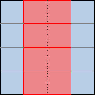
Now, as the diagram above hints, if we stacked enough sugroups on top of each other like this, we could end up having the opposite problem where our subgroups are very narrow in the horizontal direction. Which in turn could lead to worse cached data reuse across subgroups in the horizontal direction and more wasted GPU scheduler work on the bottom edge of the simulation domain.

But this is unlikely to be a problem for real-world GPUs as of 2025 because…

• As the GPUinfo database told us earlier, most GPUs have a rather wide subgroup size. 32 work-items is the most common configuration as of 2025, while 64 work-items remains quite frequent too due to its use in older AMD GPU architectures.
• 80% of GPUs whose properties were reported to GPUinfo in the past 2 years have a maximal work-group size of 1024 work-items, with a few extending a bit beyond up to 2048 work-items. With a subgroup size of 32 work-items, that’s respectively 32 and 64 subgroups, getting us close to the square-ish shape that is best for cache locality and execution efficiency.

…and if it becomes a problem for future GPUs, we will be able to address it with only slightly more complex spatial layout logic in our compute shaders:

• If subgroups end up getting narrower with respect to workgroups, then we can use a mixture of our old and new strategy to tile subgroups spatially in a 2D fashion, e.g. get 2 overlapping columns of subgroups instead of one single stack.
• If subgroups end up getting wider with respect to workgroups, then we can make a single subgroup process 2+ lines of output by using a more complicated shuffling and masking pattern that treats the subgroup as e.g. a 16x2 row-major rectangle of work-items.⁹

Sticking with simple subgroup stacking logic for now, the GLSL compute shader change is pretty straightforward as we only need to adjust the work_item_pos() function…

// To be changed in exercises/src/grayscott/step.comp

// Position of the simulation dataset that corresponds to the central value
// that this work-item will eventually write data to, if it ends up writing
uvec2 work_item_pos() {
    const uint first_x = DATA_START_POS.x - BORDER_SIZE;
    const uint item_x = gl_WorkGroupID.x * subgroup_output_size()
                        + gl_SubgroupInvocationID
                        + first_x;
    const uint item_y = gl_WorkGroupID.y * gl_NumSubgroups
                        + gl_SubgroupID
                        + DATA_START_POS.y;
    return uvec2(item_x, item_y);
}

…and on the host size, we need to adjust the compute dispatch size so that it spawns more workgroups on the horizontal axis and less on the vertical axis:

// To be changed in exercises/src/grayscott/mod.rs

/// Record the commands needed to run a bunch of simulation iterations
fn schedule_simulation(
    options: &RunnerOptions,
    context: &Context,
    pipelines: &Pipelines,
    concentrations: &mut Concentrations,
    cmdbuild: &mut CommandBufferBuilder,
) -> Result<()> {
    // [ ... everything up to subgroups_per_workgroup is unchanged ... ]
    let workgroups_per_row = options.num_cols.div_ceil(subgroup_output_size as usize) as u32;
    let workgroups_per_col = options.num_rows.div_ceil(subgroups_per_workgroup as usize) as u32;
    let simulate_workgroups = [workgroups_per_row, workgroups_per_col, 1];

    // [ ... rest is unchanged ... ]
}

And with just these two changes, we already get a better chance that our compute pipeline will experience good cache locality for loads from all directions, without relying on our GPU to “accidentally” schedule workgroups with consecutive Y coordinates on the same compute unit.

TODO: Add and comment benchmark results

Shared memory, take 2

Because a workgroup is fully processed by a single GPU compute unit, making our workgroups process a 2D chunk of the simulation dataset has significantly increased the odds that our redundant memory loads for top/bottom data points will be correctly handled by the fastest layer of cache within said compute unit, instead of taking the slow trip to VRAM.

But we cannot yet guarantee that this will happen, because workgroups are processed in parallel and a single compute unit processes multiple workgroups concurrently. Which means that unlucky GPU task scheduling could still degrade the efficiency of this automatic input data caching.

If needed, we can eliminate this last bit of reliance on lucky GPU scheduling by doing the following:

• Allocate some shared memory to make sure that the GPU reserves some cache estate for our inputs, where they cannot be displaced by unrelated loads and store, restricting the number of concurrent workgroups as much as necessary to make everything fit in cache.
• Make each work-item load its designated (U, V) pair into this cache.
• Use a workgroup barrier to wait for all input data to have been loaded into this manually managed cache, before we start reading from it.
• Read back (U, V) pairs of the top/bottom neighbors of the active work-item, if any, from the shared memory cache that we have just filled up. If we don’t have a top/bottom neighbor in the workgroup, read out top/bottom data from (possibly cached) main memory instead.

This logic is somewhat similar to what we did in the shared memory chapter, but with one important difference. In the shared memory chapter, we used to dedicate a whole row of work-items to load inputs at the top and bottom of the workgroup, in order to avoid introducing divergent “load from main memory” logic that could slow down the whole SIMD set of work-items…

…but now that our processing is subgroups-aware and our subgroup spatial layout is well controlled, we do not need to exclude that many work-items from later processing anymore.

Instead, we can simply branch and conditionally do the slow top/bottom data load when we are the top/bottom subgroup. Since subgroups are executed independently by the GPU, doing so will not slow down the rest of the workgroup. Due to this, a workgroup of the same size can process a larger output region within the simulation domain:

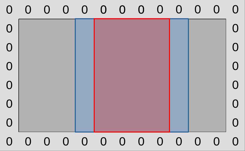
In terms of code, we can handle all of this in GLSL alone, without host involvement. First of all, we define a shared memory cache similar to the one that we had before, but this time we only allow for a vertical source data offset at load time since subgroups will take care of horizontal data motion:

// To be added to exercises/src/grayscott/step.comp, before main()

// Shared memory storage for inter-subgroup data exchange
shared float uv_cache[2][WORKGROUP_SIZE];

// Save the (U, V) value that this work-item loaded so that the rest of the
// workgroup may later access it efficiently
void set_uv_cache(vec2 uv) {
   uv_cache[U][gl_LocalInvocationID.x] = uv.x;
   uv_cache[V][gl_LocalInvocationID.x] = uv.y;
}

// Get an (U, V) value that was previously saved by a neighboring work-item
// within this workgroup. Remember to use a barrier() first!
vec2 get_uv_cache(int y_offset) {
   const int shared_pos = int(gl_LocalInvocationID.x) + y_offset * int(gl_SubgroupSize);
   return vec2(
        uv_cache[U][shared_pos],
        uv_cache[V][shared_pos]
    );
}

We then adjust the beginning of our shader entry point to load designated inputs into shared memory, as we did in the previous chapter. As before, we need to be careful not to let work-items exit too early in this version, as we will need all work-items from the workgroup in order to perform the workgroup barrier at the end.

// Simulation step entry point
void main() {
    // Map work items into 2D dataset
    const uvec2 pos = work_item_pos();

    // Load and share our designated (U, V) value, if any
    vec2 uv = vec2(0.0);
    const bool is_valid_input = all(lessThan(pos, padded_end_pos()));
    if (is_valid_input) {
        uv = read(pos);
        set_uv_cache(uv);
    }

    // Wait for the shared (U, V) cache to be ready, then discard work-items
    // that are out of bounds for input loading work.
    barrier();
    if (!is_valid_input) return;

    // [ ... more to come ... ]

We then refactor the loop over vertical neighbor coordinates so that it works using relative neighbor offsets, which are more consistent with our new logic, and then we load neighboring data from shared memory when possible and from main memory otherwise.

    for (int y = -1; y <= 1; ++y) {
        // Get the top/center/bottom value
        vec2 stencil_uvs[3];
        if (y == 0) {
            // We loaded the center value ourselves
            stencil_uvs[1] = uv;
        } else {
            // Check if the top/bottom value was read by another subgroup within
            // the current workgroup and stored back into the shared mem cache
            int target_subgroup = int(gl_SubgroupID) + y;
            if (target_subgroup >= 0 && target_subgroup < gl_NumSubgroups) {
                // If so, get it from shared memory
                stencil_uvs[1] = get_uv_cache(y);
            } else {
                // If not, perform a normal memory load
                stencil_uvs[1] = read(uvec2(
                    pos.x,
                    uint(int(pos.y) + y)
                ));
            }
        }

        // [ ... more to come ... ]
    }

Finally due to the change of y indexing convention, we need to adjust the one line of code that loads the stencil weight within the inner loop over horizontal coordinates:

        // Add associated contributions to the stencil
        for (int x = 0; x < 3; ++x) {
            const float weight = weights[x][y+1];
            full_uv += weight * (stencil_uvs[x] - uv);
        }

And with that, we will be using shared memory for manual caching again, and are ready to check again if this time the manually managed shared memory manages to outperform the automatic caching that the device automatically performs for us.

Exercise

Implement the above optimizations, and see how worthwhile they are on your device. Consider following the steps above one by one (1D workgroups, then 2D layout, then shared memory), running the microbenchmark each time to see what the impact of each optimization is: depending on how lucky/unlucky you get with GPU scheduling and caching, the outcomes may be quite different on your GPU than on the author’s!

1. Streaming Multiprocessors in NVidia jargon. ↩

2. In the interest of simplification we will ruthlessly ignore the existence of scalar GPU instructions. ↩

3. This is similar to hyperthreading on x86 CPUs, but much more important for GPU performance. The reason is that whenever there is a hardware tradeoff between execution latency and throughput, GPUs tends to favor throughput over latency. And as a result, GPU instructions tend to have much worse latency than CPU ones, especially where VRAM accesses get involved. ↩

4. Namely excellent support for gather/scatter memory access patterns and predicated conditional execution, where code that has aligned/contiguous memory access patterns and uniform logic is executed as efficiently as if these convenience/flexibility features were not there. ↩

5. Surprisingly recent, in fact, when you realize how long proprietary GPU APIs and extensions have been providing explicit SIMD instructions. For NVidia at least, shuffle support can be traced back to the Kepler microarchitecture from 2012. ↩

6. Vulkan specifies both relative and absolute shuffle operations. The former allow you to get data from the SIMD lane that is located N lanes before/after the active lane, while the latter allow you to get data from an arbitrary SIMD lane. Relative shuffles are more amenable to efficient hardware implementation, a better match for our use case, and supported on all hardware that supports shuffles at all according to the GPUinfo database, so we will go for that. ↩

7. Technically we could support unidirectional communication inside of even smaller 2-element subgroups. But GPUinfo tells us that all hardware that has more than 1 subgroup element has at least 4 of them so we don’t need to go through this trouble. ↩

8. Normally, a square-ish 2D workgroup size ensures that a maximal amount of input data points which are loaded by some work-items, and thus end up resident in the compute unit’s cache, are made available for use by neighboring work-items in the workgroup. With 1D workgroup, this is only guaranteed for left/right neighbors, not top/bottom neighbors, so we would expect worse cache locality. But we should not forget that a GPU compute unit concurrently executes many workgroups. If the GPU’s scheduler happens to schedule workgroups in such a way that workgroups associated with the same section of consecutive rows of the simulation domain are scheduled on the same compute unit, then the same kind of cache locality that we had before by construction, can happen again by luck. Now, relying on this kind of luck is not great, given that the workgroup schedulers of different GPU manufacturers are not guaranteed to all work in the same way, and that is why we will want to find a trick to enforce 2D good cache locality again even when subgroup peculiarities force us into using 1D workgroups. ↩

9. This strategy could also give us faster shuffles on modern AMD GPUs, where shuffles over 8-16 work-items get a hardware fast path compared to shuffles that cover an entire subgroups. But that comes at the expense of reduced execution efficiency (less work-items that generate and write outputs per subgroup), and in the interest of encouraging GPU code portability we would rather not put excessive emphasis on such hardware-specific optimization strategies in this course. ↩

Thread coarsening

TODO: Conclude on subgroups + shared memory with final benchmark

Overall, so far, our experiments with GPU shared memory have not been very conclusive. Sometimes a small benefit, sometimes a net loss, never a big improvement.

As discussed before, this could come from several factors, which we are unfortunately not able to disambiguate with vendor profiling tools yet:

• It might be the case that the scheduling and caching stars aligned just right on our first attempt, and that we got excellent compute unit caching efficiency from the beginning. If so, it is normal that replacing the compute unit’s automatic caching with manual shared memory caching does not help performance much, as we’re using a more complex GPU program just to get the same result in the end.
• Or it might be the case that we are hitting a bottleneck related to our use of shared memory, which may originate from an unavoidable limitation of the hardware shared memory implementation, or from the way we use shared memory in our code.

Now that we have covered subgroups, we are ready to elaborate on the “hardware limitation” part. As of 2025, most recent GPUs from AMD and NVidia use compute units that contain four 32-lanes SIMD ALUs (or 128 SIMD lanes in total), but only 32 shared memory banks, each of which can load or store one 32-bit value per clock cycle.

Knowing these microarchitectural numbers, we can easily tell in situations where all active workgroups are putting pressure on shared memory, associated load/store instructions only execute at a quarter of the rate compared with arithmetic operations. This could easily become a bottleneck in memory-intensive computations like ours.

And if this relatively low hardware load/store bandwidth turns out to be the factor that limits our performance, then the answer is to use a layer of the GPU memory hierarchy that is even faster than shared memory. And the choice will be easy here, since there is only one option here that is user-accessible in portable GPU APIs, namely GPU registers.

Leveraging registers

GPU vector registers are private to a subgroup, and there is no way to share them across subgroups. In fact the only interface that we GPU programmers have to allocate and use registers are shader local variables, which are logically private to the active work-item. In normal circumstances,¹ each local 32-bit variable from a shader, which has a value that will be reused later by the program, maps into one lane of a vector register, owned by the subgroup that the active work-item belongs to.

Any data that is cached within GPU registers must therefore be reused by either the same work-item, or another work-item within the same subgroup. The previous chapter was actually our first example of the latter. In it, work-items were able to share data held inside of their vector registers without going through shared memory by leveraging subgroup operations. On typical GPU hardware, those operations are implemented in a such a way that everything goes through GPU registers and shared memory storage banks do not get involved.

But subgroup operations are mostly useful for sharing data over a one-dimensional axis, and attempting to use them for two-dimensional data sharing would likely not work so well because we would need to reserve too many work-items for input loading purposes and thus lose too much compute throughput during the arithmetic computations.

To convince yourself of this, recall that right now, assuming the common case of 32-lane subgroups, we only need need to reserve one work-item on the left and one on the right for input loading, which only costs us 2/32 = 6.25% of our SIMD arithmetic throughput during the main computation.

If we rearranged that same 32-lane subgroup into a 8x4 two-dimensional shape, then reserving one work-item on each side for input loading would only leave us with 2x6 = 12 work-items in the middle for the rest of the computation. In other words, we would have sacrificed 20/32 = 62.5% of our available compute throughput to our quest for faster data loading, which feels excessive…

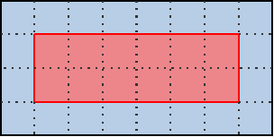
…and as discussed before, we need this reserved input on each side for subgroup-based sharing to be worthwhile. If the work-items on the edge simply loaded missing neighbor data from main memory and proceeded with the reste of the computation, then the entire subgroup would become bottlenecked by the performance of loading these neighbors from main memory due to lockstep SIMD execution, nullifying most of the benefits of fast data sharing inside of the subgroup.

However, there is an alternative to using subgroups for efficient data sharing across the vertical axis. We can keep our subgroups focused on the processing of horizontal lines, but have each subgroup process multiple lines of input/output data instead of a single one. In this situation, if each individual subgroup keeps around a circular buffer of the last three lines of input that it has been reading (which will be stored in GPU vector registers), then for each new line of outputs after the first one, that subgroup will be will be loading only the next line of input from main GPU memory, while the other two lines of inputs will be loaded from fast vector registers.

This may be a bit too much textual info at once, so let’s visualize it in pictures:

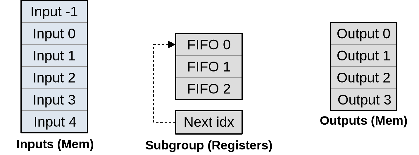
As summarized on the diagram above, our subgroup has a set of input memory locations forming a vertical stack, a set of output memory locations also forming a vertical stack but with two lines less, and an internal circular buffer composed that is composed of…

• An array of three (U, V) inputs per work-item (or triplets thereof if left/right neighbors are cached to avoid repeated shuffling) that will be used to store a rolling window of input data during subsequent processing.
• An integer that indicates where input will be loaded next.

As part of work item initialization, we prepare the processing pipeline by loading the first two lines of lines of input into the circular buffer, incrementing its next location index accordingly:

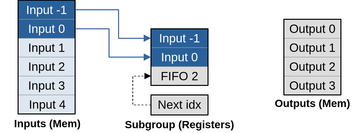
Once this is done, we can produce the first input by loading another input into the circular buffer, then using all three circular buffer entries to produce the output…

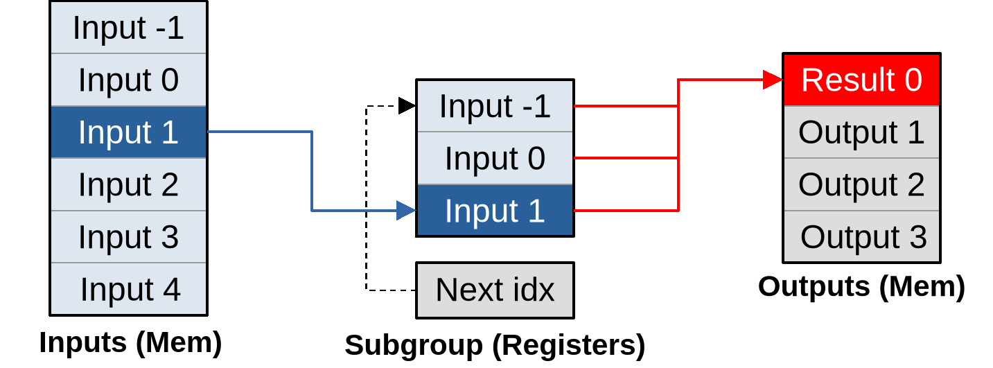
…and the whole point of going through this more complex logic is that after doing that, for each new vector of inputs that load, our subgroup can immediately produce another vector of outputs:

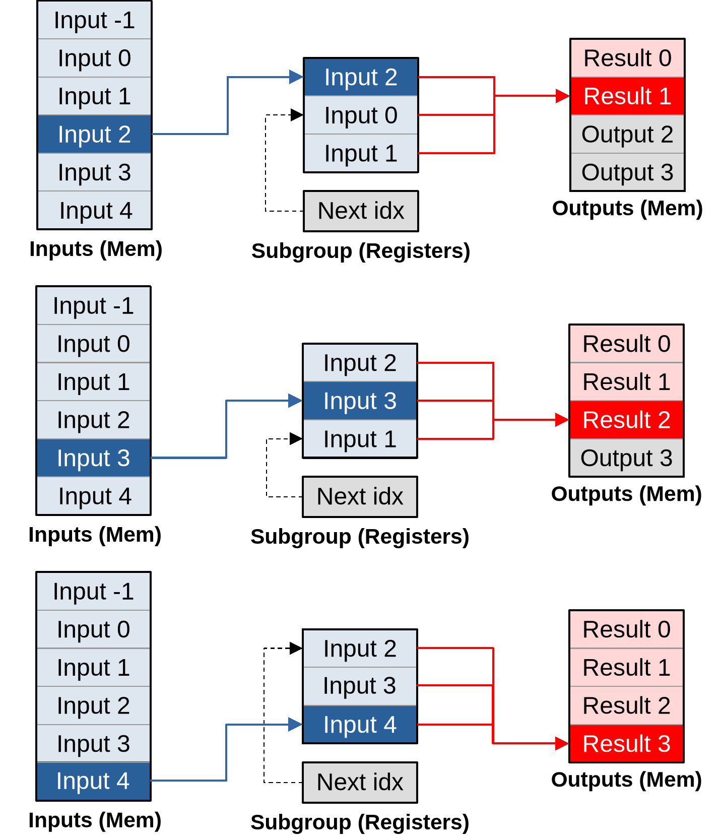
As you can see, given a large enough outputs per work item, this pipeline converges to an optimal asymptotic efficiency of loading one vector of inputs per vector of outputs that is being produced.

And that is not the only benefit of doing things this way. Because we are doing more work per work-item, we will also be able to amortize the hardware costs associated with spawning a work-group on the GPU, and the software costs of initializing each work-item from it on our side. For example…

• Since we know that a subgroup will be producing consecutive lines of output, we will only need to call the relatively complex work_item_pos() GLSL function once, and will be able to simply increment the Y coordinate of the resulting position vector for each subsequent input.
• Since the X coordinate targeted by the subgroup does not change, we will only need to check if that X coordinate is out of bounds once, and all subsequent calculations will simply need to check that the target Y output coordinate is still in bounds.
• If the GPU’s instruction set is not able to encode the matrix of stencil weights and other constants into immediate instruction operands, and must load them from some compute unit local constant cache with finite bandwidth, then after this change we will only need to load these constants once, and can keep them around in scalar GPU registers afterwards for faster access in all subsequent output computations.

The bad news

All of the above may all sound pretty amazing, at at this point you may be wondering why I have not introduced this optimization earlier in this course. But in software performance engineering, there is rarely such a thing as a perfect optimization strategy that has only upsides and no downsides.

This particular optimization strategy is no exception, as its many upsides come at the expense of two very important downsides, which are the reasons why it is usually only tried as a last resort:

• Reduced concurrency: If each GPU work-item does more work, it means that we use less work-items to do the same amount of work, and thus we feed the GPU with fewer concurrent tasks. But GPUs need plenty of concurrent tasks to fill up their compute units and hide the latency of individual operations, and the more powerful they are the worst this gets. So overall this optimization may decrease our program’s ability to efficiently utilize larger, higher-end GPUs, at equal domain size. And conversely we will need to simulate larger simulation domains in order to achieve the same computational efficiency on a particular GPU.
• Register pressure: Everything mentioned so far relies on the GPU compiler keeping a lot more state in registers than before, without being able to discard this state immediately after use because it will be reused when producing the next GPU output. This will result in “bigger” GPU workgroups with a larger register footprint, potentially making us hit the hardware limit where a GPU is not able to fill compute units with workgroups up to their maximal capacity anymore. Given fewer concurrent workgroups, compute units get worse at latency hiding, which means that we will need to be more careful with avoiding high-latency operations. If we take this too far, the GPU won’t even be able to fill up a compute unit with enough work to keep all of its SIMD ALUs active, and then performance will fall down a cliff.

Without orders of magnitude, these two issues may sound abstract and perhaps too minor to worry about. So let’s get some numbers from the author’s Radeon RX 5600M GPU, which has been used to produce most benchmark data featured in this course.

Some concurrency numbers

This GPU implements the first-generation AMD RDNA architecture, which comes with reasonable first-party ISA and microarchitecture documentation, as well as a handy device comparison table from some great Wikipedia editors.

The Wikipedia data tells us that the RX 5600M has 36 compute unit, which the microarchitecture documentation tells us each contain two 32-lane SIMD units that can each manage 20 concurrent workgroups for latency hiding. This means that an absolute minimum of 36x2x32 = 2304 work-items is required to use the GPU’s full parallel processing capabilities.

For optimal latency hiding you will want 20 times that (46080 work-items). And for other reasons like load balancing and amortizing the fixed costs of initializing a compute dispatch, peak processing efficiency is typically not reached until a 10~100x larger number of work-items are used. This is where the “GPU needs millions of threads” meme come from.

From this perspective, we can see that our initial compute dispatch size of 1920x1080 ~ 2 million work-items is not that big, and we should be careful about reducing it too much. And this is on a mid-range laptop GPU from several years ago. More recent and higher-end GPUs have even more parallelism, and will therefore suffer more from a reduction of work-item concurrency.

Some register pressure numbers

As for registers, elsewhere in the RDNA microarchitectural documentation, we find that each SIMD ALU has access to 1024 vector registers with 32-bit lanes. Given that this SIMD ALU manages up to 20 concurrent workgroups, this means that in a maximal-concurrency configuration, each workgroup may only use up to 51 32-bit registers of per work-item state. And the actual register budget is actually even less than that, because some of these registers are used to store microarchitectural state such as the index of the current work-group within the dispatch and that of the current subgroup within the workgroup.

To those who come from an x86 CPU programming world, where 16 SIMD registers has been the norm for a long time and 32 registers is a shiny recent development, 50 registers may sound plentiful. But x86 CPUs also enjoy much faster L1 caches. A modern x86 CPU that processes 2 vector FMAs per clock cycle can also process at least 2 L1 vector loads and 1 L1 vector store per clock cycle, which means that the ratio between arithmetic and caching capacity is a lot more balanced than on GPU, where the fastest available memory operations execute at quarter rate compared to FMAs.

And that difference in arithmetic/memory performance balance is why on x86 CPUs occasional spilling of SIMD registers to the stack is not considered a performance problem outside of the hottest inner loops, whereas on GPU much more effort is expended on getting programs that never need to spill register state to shared memory, let alone main memory.

Back to the algorithm above, if we choose to keep around the past two (U, V) inputs, and for each input also cache the left and right neighbor of the active data point to save on shuffle operations, then this optimization alone is going to increase the vector register footprint of each work-item by 2x2x3 = 12 registers, which on its own eats 1/4 of our per work-item register budget at maximal workgroup concurrency. And most of the other state caching optimizations that we discussed before would require a few more registers each.

So as you can see, it it not that we can never do such optimizations, but we must be very careful about not running out of registers when we do so. If we run out of registers, then the GPU hardware will end up either reducing workgroup concurrency or spilling registers to main memory, and in either case our optimization is likely to hurt performance more than it helps.

Implementation

Before applying this optimization, we will revert the two previous ones that introduced a 2D workgroup layout and usage of shared memory, and instead go back to the 1D workgroups that we had at the beginning of the subgroup chapter. Here is why:

• Before, we had a clear “current input” to cache. Now we need to cache the first and last input from the input sequence. That would make us use twice the amount of cache/shared memory footprint and bandwidth, when those resources have not performed well so far.
• Shared memory and caches could be faster on other current and future GPUs, which would be an argument for keeping the previous optimization if it does not harm much. But if this new optimization works, the performance impact of shared memory will become smaller in both directions. The more inputs we process per work-item, the less of an impact caching the first/last input of each work-item will have.
• To make those first/last inputs quickly available to other GPU work-items, so that they can reuse them, we need to read them first. This means reading inputs out of order, and the prefetchers of GPU memory hierarchies are likely to get confused by this irregular access pattern and behave less well as a result.

This means that on the GLSL side, our work-item positioning logic will go back to the following…

// Change in exercises/src/grayscott/step.comp

// Maximal number of output data points per workgroup (see above)
uint workgroup_output_size() {
    return gl_NumSubgroups * subgroup_output_size();
}

// Position of the simulation dataset that corresponds to the central value
// that this work-item will eventually write data to, if it ends up writing
uvec2 work_item_pos() {
    const uint first_x = DATA_START_POS.x - BORDER_SIZE;
    const uint item_x = gl_WorkGroupID.x * workgroup_output_size()
                        + gl_SubgroupID * subgroup_output_size()
                        + gl_SubgroupInvocationID
                        + first_x;
    const uint item_y = gl_WorkGroupID.y + DATA_START_POS.y;
    return uvec2(item_x, item_y);
}

…and our diffusion gradient computation will go back to the following…

void main() {
    // Map work items into 2D dataset, discard those outside input region
    // (including padding region).
    const uvec2 pos = work_item_pos();
    if (any(greaterThanEqual(pos, padded_end_pos()))) {
        return;
    }

    // Load central value
    const vec2 uv = read(pos);

    // Compute the diffusion gradient for U and V
    const uvec2 top = pos - uvec2(0, 1);
    const mat3 weights = stencil_weights();
    vec2 full_uv = vec2(0.0);
    for (int y = 0; y < 3; ++y) {
        // Read the top/center/bottom value
        vec2 stencil_uvs[3];
        stencil_uvs[1] = read(top + uvec2(0, y));

        // Get the left/right value from neighboring work-items
        //
        // This will be garbage data for the work-items on the left/right edge
        // of the subgroup, but that's okay, we'll filter these out with an
        // is_subgroup_output() condition later on.
        //
        // It can also be garbage on the right edge of the simulation domain
        // where the right neighbor has been rendered inactive by the
        // padded_end_pos() filter above, but if we have no right neighbor we
        // are only loading data from the zero edge of the simulation dataset,
        // not producing an output. So our garbage result will be masked out by
        // the other pos < data_end_pos() condition later on.
        stencil_uvs[0] = shuffle_from_left(stencil_uvs[1]);
        stencil_uvs[2] = shuffle_from_right(stencil_uvs[1]);

        // Add associated contributions to the stencil
        for (int x = 0; x < 3; ++x) {
            full_uv += weights[x][y] * (stencil_uvs[x] - uv);
        }
    }

    // [ ... rest is unchanged ... ]
}

…while on the Rust side our dispatch size computation will go back to the following:

// Change in exercises/src/grayscott/mod.rs

fn schedule_simulation(
    options: &RunnerOptions,
    context: &Context,
    pipelines: &Pipelines,
    concentrations: &mut Concentrations,
    cmdbuild: &mut CommandBufferBuilder,
) -> Result<()> {
    // [ ... steps up to subgroups_per_workgroup computation are unchanged ... ]
    let outputs_per_workgroup = subgroups_per_workgroup * subgroup_output_size;
    let workgroups_per_row = options.num_cols.div_ceil(outputs_per_workgroup as usize) as u32;
    let simulate_workgroups = [workgroups_per_row, options.num_rows as u32, 1];

    // [ ... rest is unchanged ... ]
}

After doing this, we will add a new specialization constant to our compute pipelines,

TODO: Describe the code and try it at various sizes. Try other subgroup reconvergence models to see if they help. Analyze register pressure before/after using RGA.

1. If a GLSL shader has so many local variables that they cannot all be kept into hardware registers, the GPU scheduler will first try to spawn less workgroups per compute unit. If even that does not suffice, then the GPU compiler may decide to do what a CPU compiler would do and spill some of these variables to local caches or main GPU memory. This is usually very bad for performance, so GPU programmers normally take care not to get into this situation. ↩

Kernel fission

TODO: Reword based on preceding chapters

In the previous chapters, we have been implementing code optimizations that make more parts of our simulation execute in parallel through a mixture of asynchronous execution and pipelining.

As a result, we went from a rather complex situation where our simulation speed was limited by various hardware performance characteristics depending on the configuration in which we executed it, to a simpler situation where our simulation is more and more often bottlenecked by the raw speed at which we perform simulation steps.

This is shown by the fact that in our reference configuration, where our simulation domain contains about 2 billion pixels and we perform 32 simulation steps per generated image, the simulation speed that is measured by our microbenchmark does not change that much anymore as we go from a pure GPU compute scenario to a scenario where we additionally download data from the GPU to the CPU and post-process it on the CPU:

run_simulation/workgroup32x16/domain2048x1024/total512/image32/compute
                        time:   [83.137 ms 83.266 ms 83.421 ms]
                        thrpt:  [12.871 Gelem/s 12.895 Gelem/s 12.915 Gelem/s]
run_simulation/workgroup32x16/domain2048x1024/total512/image32/compute+download
                        time:   [102.03 ms 102.49 ms 102.95 ms]
                        thrpt:  [10.429 Gelem/s 10.477 Gelem/s 10.524 Gelem/s]
run_simulation/workgroup32x16/domain2048x1024/total512/image32/compute+download+sum
                        time:   [102.98 ms 103.21 ms 103.36 ms]
                        thrpt:  [10.389 Gelem/s 10.404 Gelem/s 10.427 Gelem/s]

To go faster, we will therefore need to experiment with ways to make our simulation steps faster. Which is what the next optimization chapters of this course will focus on.

As a first step, we will try a classic GPU optimization strategy: when given the choice between more concurrent work and less redundant work, always try more concurrency first.

A concurrency opportunity

Recall that our GPU program for performing a simulation step looks like this:

void main() {
    // Map work items into 2D central region, discard out-of-bounds work items
    const uvec2 pos = uvec2(gl_GlobalInvocationID.xy) + DATA_START_POS;
    if (any(greaterThanEqual(pos, data_end_pos()))) {
        return;
    }

    // Load central value
    const vec2 uv = read(pos);

    // Compute the diffusion gradient for U and V
    const uvec2 topleft = pos - uvec2(1);
    const mat3 weights = stencil_weights();
    vec2 full_uv = vec2(0.0);
    for (int y = 0; y < 3; ++y) {
        for (int x = 0; x < 3; ++x) {
            const vec2 stencil_uv = read(topleft + uvec2(x, y));
            full_uv += weights[x][y] * (stencil_uv - uv);
        }
    }

    // Deduce the change in U and V concentration
    const float u = uv.x;
    const float v = uv.y;
    const float uv_square = u * v * v;
    const vec2 delta_uv = diffusion_rate() * full_uv + vec2(
        FEED_RATE * (1.0 - u) - uv_square,
        uv_square - (FEED_RATE + KILL_RATE) * v
    );
    write(pos, uv + delta_uv * DELTA_T);
}

If you look at it carefully, you will realize that it is almost two computations bundled into one:

• The initial full_uv diffusion gradient computation independently computes the diffusion gradient for species U and V, as two different lanes of a GLSL vec2 type.
• The final delta_uv computation is literally two different computations vectorized into one, with the exception of the uv_square product which is only computed once but used by the U and V components of delta_uv.

As it turns out, GPU hardware isn’t very good at this sort of explicit vectorization,¹ and GLSL vector types like vec2 are more useful for ergonomics than for performance. Therefore, in case our computation doesn’t have enough internal concurrency to saturate the GPU’s compute units (which is likely to be the case on higher-end GPUs) , we may benefit from splitting this computation into two, one for U and one for V, even though this will come at the expense of a bit of redundant work.

Indeed, there is a price to pay for the extra concurrency enabled by this alternate strategy, which is that the computation for one chemical species will need to load the central value of the other species and to perform a pair of multiplications in order to compute the uv_square product.

Separating the U and V computations

In the common.comp GLSL source file, which contains code shared between our compute shaders, we will supplement the existing read() and write() functions with alternatives that only read and write a single species’ concentration…

// Read U or V from a particular input location, pos works as in read()
float read_one(uint species, uvec2 pos) {
    const uint index = pos_to_index(pos);
    return Input[species].data[index];
}

// Write U or V to a particular output location, pos works as in read()
void write_one(uint species, uvec2 pos, float value) {
    const uint index = pos_to_index(pos);
    Output[species].data[index] = value;
}

…and we will extract a variation of our former diffusion gradient computation that only performs the computation for a single chemical species:

// Diffusion gradient computation for a single species
float diffusion_gradient(uint species, uvec2 pos, float center_value) {
    const uvec2 topleft = pos - uvec2(1);
    const mat3 weights = stencil_weights();
    float gradient = 0.0;
    for (int y = 0; y < 3; ++y) {
        for (int x = 0; x < 3; ++x) {
            const float stencil = read_one(species, topleft + uvec2(x, y));
            gradient += weights[x][y] * (stencil - center_value);
        }
    }
    return gradient;
}

Given this infrastructure, we will be able to write a compute shader that only computes the concentration of the U species, which we will save to a file called step_u.comp…

#version 460

#include "common.comp"

// Simulation step entry point for the U species
void main() {
    // Map work items into 2D central region, discard out-of-bounds work items
    const uvec2 pos = uvec2(gl_GlobalInvocationID.xy) + DATA_START_POS;
    if (any(greaterThanEqual(pos, data_end_pos()))) {
        return;
    }

    // Load central value of U and V
    const vec2 uv = read(pos);
    const float u = uv.x;
    const float v = uv.y;

    // Compute the diffusion gradient for U
    const float full_u = diffusion_gradient(U, pos, u);

    // Deduce the change in U concentration
    const float uv_square = u * v * v;
    const float delta_u = DIFFUSION_RATE_U * full_u
                          - uv_square
                          + FEED_RATE * (1.0 - u);
    write_one(U, pos, u + delta_u * DELTA_T);
}

…and another compute shader that only computes the concentration of the V species, which we will save to a fille called step_v.comp…

#version 460

#include "common.comp"

// Simulation step entry point for the V species
void main() {
    // Map work items into 2D central region, discard out-of-bounds work items
    const uvec2 pos = uvec2(gl_GlobalInvocationID.xy) + DATA_START_POS;
    if (any(greaterThanEqual(pos, data_end_pos()))) {
        return;
    }

    // Load central value of U and V
    const vec2 uv = read(pos);
    const float u = uv.x;
    const float v = uv.y;

    // Compute the diffusion gradient for V
    const float full_v = diffusion_gradient(V, pos, v);

    // Deduce the change in V concentration
    const float uv_square = u * v * v;
    const float delta_v = DIFFUSION_RATE_V * full_v
                          + uv_square
                          - (FEED_RATE + KILL_RATE) * v;
    write_one(V, pos, v + delta_v * DELTA_T);
}

…without suffering an unbearable amount of GLSL code duplication between these two compute shaders, though there will obviously be similarities.

Adapting the CPU code

To support this new style of computation, we will need to extend our pipeline.rs module so that it builds two compute pipelines instead of one. This can be done by adjusting our vulkano_shaders::shader macro call to cover the two new step_u and step_v compute shaders…

/// Shader modules used for the compute pipelines
mod shader {
    vulkano_shaders::shader! {
        shaders: {
            init: {
                ty: "compute",
                path: "src/grayscott/init.comp"
            },
            step_u: {
                ty: "compute",
                path: "src/grayscott/step_u.comp"
            },
            step_v: {
                ty: "compute",
                path: "src/grayscott/step_v.comp"
            },
        }
    }
}

…and adjusting the Pipelines struct and its constructor in order to build this new pair of compute pipelines, where it used to build a single step compute pipeline before:

/// Initialization and simulation pipelines with common layout information
#[derive(Clone)]
pub struct Pipelines {
    /// Compute pipeline used to initialize the concentration tables
    pub init: Arc<ComputePipeline>,

    /// Compute pipeline used to perform a simulation step for U
    pub step_u: Arc<ComputePipeline>,

    /// Compute pipeline used to perform a simulation step for V
    pub step_v: Arc<ComputePipeline>,

    /// Pipeline layout shared by `init` and `step`
    pub layout: Arc<PipelineLayout>,
}
//
impl Pipelines {
    /// Set up all the compute pipelines
    pub fn new(options: &RunnerOptions, context: &Context) -> Result<Self> {
        // Common logic for setting up a compute pipeline stage
        fn setup_stage_info(
            options: &RunnerOptions,
            context: &Context,
            load: impl FnOnce(
                Arc<Device>,
            )
                -> std::result::Result<Arc<ShaderModule>, Validated<VulkanError>>,
        ) -> Result<PipelineShaderStageCreateInfo> {
            let module = load(context.device.clone())?;
            let module = setup_shader_module(options, module)?;
            Ok(setup_compute_stage(module))
        }

        // Set up the initialization and step pipeline stages, making sure that
        // they share a common pipeline layout so that they can use the same
        // resource descriptor sets later on
        let init_stage_info = setup_stage_info(options, context, shader::load_init)?;
        let step_u_stage_info = setup_stage_info(options, context, shader::load_step_u)?;
        let step_v_stage_info = setup_stage_info(options, context, shader::load_step_v)?;
        let layout = setup_pipeline_layout(
            context.device.clone(),
            [&init_stage_info, &step_u_stage_info, &step_v_stage_info],
        )?;

        // Finish setting up the initialization and stepping compute pipelines
        let setup_compute_pipeline = |stage_info: PipelineShaderStageCreateInfo| {
            let pipeline_info = ComputePipelineCreateInfo::stage_layout(stage_info, layout.clone());
            ComputePipeline::new(
                context.device.clone(),
                Some(context.pipeline_cache()),
                pipeline_info,
            )
        };
        Ok(Self {
            init: setup_compute_pipeline(init_stage_info)?,
            step_u: setup_compute_pipeline(step_u_stage_info)?,
            step_v: setup_compute_pipeline(step_v_stage_info)?,
            layout,
        })
    }
}

Finally, we will modify the schedule_simulation() function so that it uses this pair of compute pipelines instead of a single compute pipeline:

/// Record the commands needed to run a bunch of simulation iterations
fn schedule_simulation(
    options: &RunnerOptions,
    pipelines: &Pipelines,
    concentrations: &mut Concentrations,
    cmdbuild: &mut CommandBufferBuilder,
) -> Result<()> {
    // [ ... compute dispatch size computation is unchanged ... ]

    // Schedule the requested number of simulation steps
    for _ in 0..options.steps_per_image {
        concentrations.update(|inout_set| {
            cmdbuild.bind_descriptor_sets(
                PipelineBindPoint::Compute,
                pipelines.layout.clone(),
                INOUT_SET,
                inout_set,
            )?;
            for pipeline in [&pipelines.step_u, &pipelines.step_v] {
                cmdbuild.bind_pipeline_compute(pipeline.clone())?;
                // SAFETY: GPU shader has been checked for absence of undefined behavior
                //         given a correct execution configuration, and this is one
                unsafe {
                    cmdbuild.dispatch(simulate_workgroups)?;
                }
            }
            Ok(())
        })?;
    }
    Ok(())
}

Exercise

Implement this optimization and measure its impact on the GPU(s) that you have access to.

On the author’s AMD Radeon RX 5600M laptop GPU, the net impact of this optimization is negative (20-30% slowdown), which means the extra concurrency that we gain is not worth the extra computational costs that we pay for. But on a higher-end GPU, the tradeoff may be different.

1. Barring exceptions like half-precision floating point numbers and special-purpose “tensor cores”. ↩