Thread coarsening

TODO: Conclude on subgroups + shared memory with final benchmark

Overall, so far, our experiments with GPU shared memory have not been very conclusive. Sometimes a small benefit, sometimes a net loss, never a big improvement.

As discussed before, this could come from several factors, which we are unfortunately not able to disambiguate with vendor profiling tools yet:

• It might be the case that the scheduling and caching stars aligned just right on our first attempt, and that we got excellent compute unit caching efficiency from the beginning. If so, it is normal that replacing the compute unit’s automatic caching with manual shared memory caching does not help performance much, as we’re using a more complex GPU program just to get the same result in the end.
• Or it might be the case that we are hitting a bottleneck related to our use of shared memory, which may originate from an unavoidable limitation of the hardware shared memory implementation, or from the way we use shared memory in our code.

Now that we have covered subgroups, we are ready to elaborate on the “hardware limitation” part. As of 2025, most recent GPUs from AMD and NVidia use compute units that contain four 32-lanes SIMD ALUs (or 128 SIMD lanes in total), but only 32 shared memory banks, each of which can load or store one 32-bit value per clock cycle.

Knowing these microarchitectural numbers, we can easily tell in situations where all active workgroups are putting pressure on shared memory, associated load/store instructions only execute at a quarter of the rate compared with arithmetic operations. This could easily become a bottleneck in memory-intensive computations like ours.

And if this relatively low hardware load/store bandwidth turns out to be the factor that limits our performance, then the answer is to use a layer of the GPU memory hierarchy that is even faster than shared memory. And the choice will be easy here, since there is only one option here that is user-accessible in portable GPU APIs, namely GPU registers.

Leveraging registers

GPU vector registers are private to a subgroup, and there is no way to share them across subgroups. In fact the only interface that we GPU programmers have to allocate and use registers are shader local variables, which are logically private to the active work-item. In normal circumstances,¹ each local 32-bit variable from a shader, which has a value that will be reused later by the program, maps into one lane of a vector register, owned by the subgroup that the active work-item belongs to.

Any data that is cached within GPU registers must therefore be reused by either the same work-item, or another work-item within the same subgroup. The previous chapter was actually our first example of the latter. In it, work-items were able to share data held inside of their vector registers without going through shared memory by leveraging subgroup operations. On typical GPU hardware, those operations are implemented in a such a way that everything goes through GPU registers and shared memory storage banks do not get involved.

But subgroup operations are mostly useful for sharing data over a one-dimensional axis, and attempting to use them for two-dimensional data sharing would likely not work so well because we would need to reserve too many work-items for input loading purposes and thus lose too much compute throughput during the arithmetic computations.

To convince yourself of this, recall that right now, assuming the common case of 32-lane subgroups, we only need need to reserve one work-item on the left and one on the right for input loading, which only costs us 2/32 = 6.25% of our SIMD arithmetic throughput during the main computation.

If we rearranged that same 32-lane subgroup into a 8x4 two-dimensional shape, then reserving one work-item on each side for input loading would only leave us with 2x6 = 12 work-items in the middle for the rest of the computation. In other words, we would have sacrificed 20/32 = 62.5% of our available compute throughput to our quest for faster data loading, which feels excessive…

…and as discussed before, we need this reserved input on each side for subgroup-based sharing to be worthwhile. If the work-items on the edge simply loaded missing neighbor data from main memory and proceeded with the reste of the computation, then the entire subgroup would become bottlenecked by the performance of loading these neighbors from main memory due to lockstep SIMD execution, nullifying most of the benefits of fast data sharing inside of the subgroup.

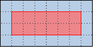
However, there is an alternative to using subgroups for efficient data sharing across the vertical axis. We can keep our subgroups focused on the processing of horizontal lines, but have each subgroup process multiple lines of input/output data instead of a single one. In this situation, if each individual subgroup keeps around a circular buffer of the last three lines of input that it has been reading (which will be stored in GPU vector registers), then for each new line of outputs after the first one, that subgroup will be will be loading only the next line of input from main GPU memory, while the other two lines of inputs will be loaded from fast vector registers.

This may be a bit too much textual info at once, so let’s visualize it in pictures:

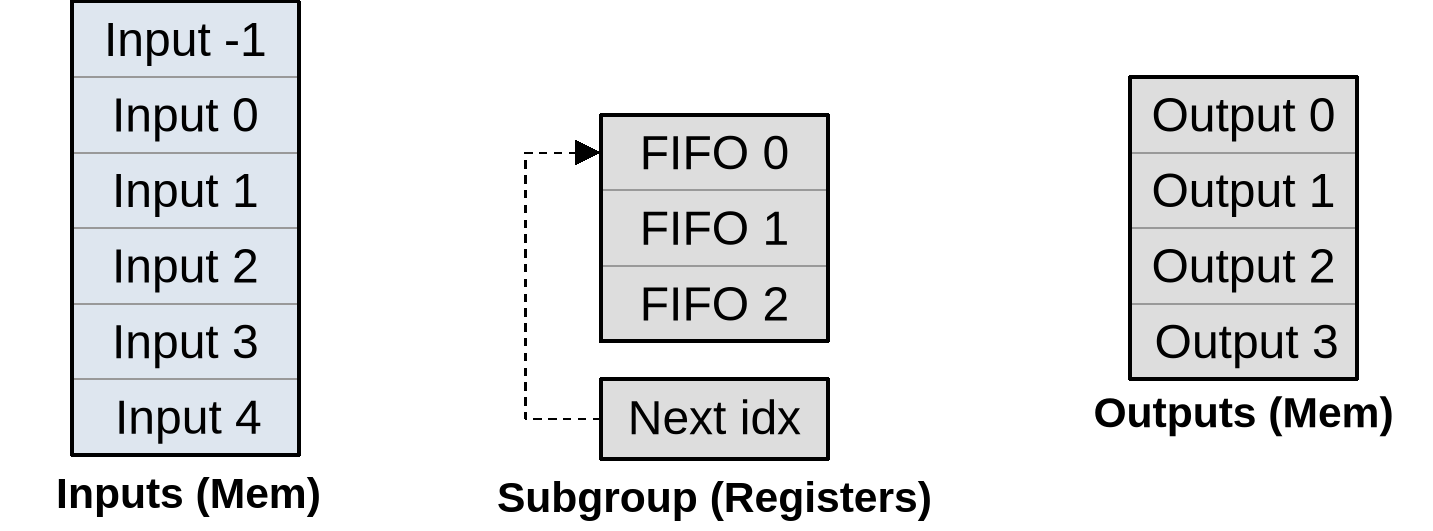
As summarized on the diagram above, our subgroup has a set of input memory locations forming a vertical stack, a set of output memory locations also forming a vertical stack but with two lines less, and an internal circular buffer composed that is composed of…

• An array of three (U, V) inputs per work-item (or triplets thereof if left/right neighbors are cached to avoid repeated shuffling) that will be used to store a rolling window of input data during subsequent processing.
• An integer that indicates where input will be loaded next.

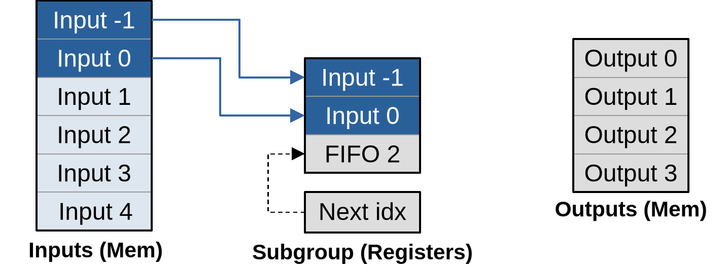
As part of work item initialization, we prepare the processing pipeline by loading the first two lines of lines of input into the circular buffer, incrementing its next location index accordingly:

Once this is done, we can produce the first input by loading another input into the circular buffer, then using all three circular buffer entries to produce the output…

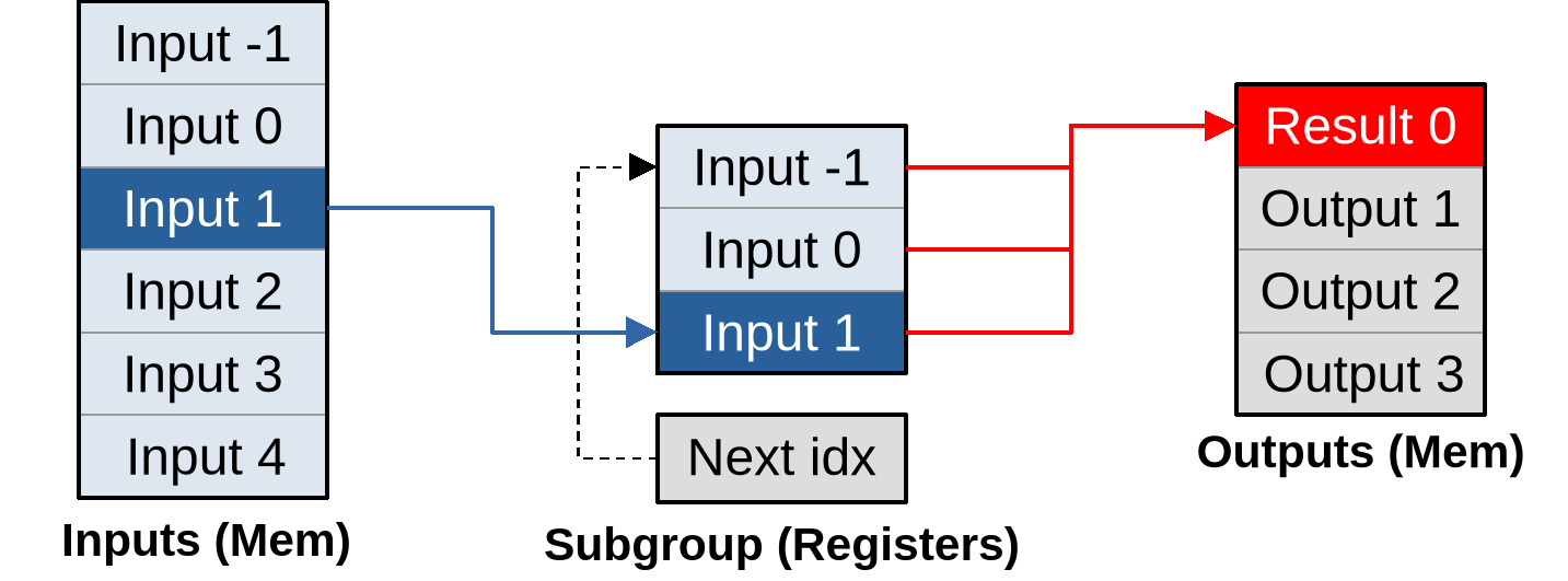
…and the whole point of going through this more complex logic is that after doing that, for each new vector of inputs that load, our subgroup can immediately produce another vector of outputs:

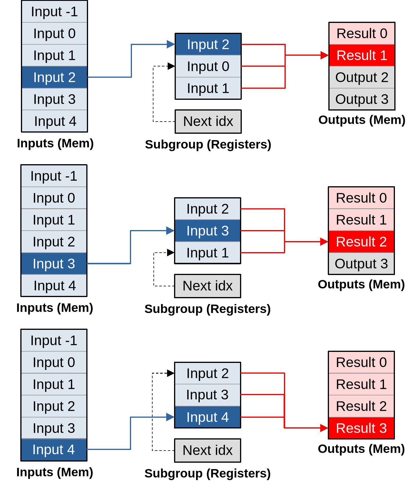
As you can see, given a large enough outputs per work item, this pipeline converges to an optimal asymptotic efficiency of loading one vector of inputs per vector of outputs that is being produced.

And that is not the only benefit of doing things this way. Because we are doing more work per work-item, we will also be able to amortize the hardware costs associated with spawning a work-group on the GPU, and the software costs of initializing each work-item from it on our side. For example…

• Since we know that a subgroup will be producing consecutive lines of output, we will only need to call the relatively complex work_item_pos() GLSL function once, and will be able to simply increment the Y coordinate of the resulting position vector for each subsequent input.
• Since the X coordinate targeted by the subgroup does not change, we will only need to check if that X coordinate is out of bounds once, and all subsequent calculations will simply need to check that the target Y output coordinate is still in bounds.
• If the GPU’s instruction set is not able to encode the matrix of stencil weights and other constants into immediate instruction operands, and must load them from some compute unit local constant cache with finite bandwidth, then after this change we will only need to load these constants once, and can keep them around in scalar GPU registers afterwards for faster access in all subsequent output computations.

The bad news

All of the above may all sound pretty amazing, at at this point you may be wondering why I have not introduced this optimization earlier in this course. But in software performance engineering, there is rarely such a thing as a perfect optimization strategy that has only upsides and no downsides.

This particular optimization strategy is no exception, as its many upsides come at the expense of two very important downsides, which are the reasons why it is usually only tried as a last resort:

• Reduced concurrency: If each GPU work-item does more work, it means that we use less work-items to do the same amount of work, and thus we feed the GPU with fewer concurrent tasks. But GPUs need plenty of concurrent tasks to fill up their compute units and hide the latency of individual operations, and the more powerful they are the worst this gets. So overall this optimization may decrease our program’s ability to efficiently utilize larger, higher-end GPUs, at equal domain size. And conversely we will need to simulate larger simulation domains in order to achieve the same computational efficiency on a particular GPU.
• Register pressure: Everything mentioned so far relies on the GPU compiler keeping a lot more state in registers than before, without being able to discard this state immediately after use because it will be reused when producing the next GPU output. This will result in “bigger” GPU workgroups with a larger register footprint, potentially making us hit the hardware limit where a GPU is not able to fill compute units with workgroups up to their maximal capacity anymore. Given fewer concurrent workgroups, compute units get worse at latency hiding, which means that we will need to be more careful with avoiding high-latency operations. If we take this too far, the GPU won’t even be able to fill up a compute unit with enough work to keep all of its SIMD ALUs active, and then performance will fall down a cliff.

Without orders of magnitude, these two issues may sound abstract and perhaps too minor to worry about. So let’s get some numbers from the author’s Radeon RX 5600M GPU, which has been used to produce most benchmark data featured in this course.

Some concurrency numbers

This GPU implements the first-generation AMD RDNA architecture, which comes with reasonable first-party ISA and microarchitecture documentation, as well as a handy device comparison table from some great Wikipedia editors.

The Wikipedia data tells us that the RX 5600M has 36 compute unit, which the microarchitecture documentation tells us each contain two 32-lane SIMD units that can each manage 20 concurrent workgroups for latency hiding. This means that an absolute minimum of 36x2x32 = 2304 work-items is required to use the GPU’s full parallel processing capabilities.

For optimal latency hiding you will want 20 times that (46080 work-items). And for other reasons like load balancing and amortizing the fixed costs of initializing a compute dispatch, peak processing efficiency is typically not reached until a 10~100x larger number of work-items are used. This is where the “GPU needs millions of threads” meme come from.

From this perspective, we can see that our initial compute dispatch size of 1920x1080 ~ 2 million work-items is not that big, and we should be careful about reducing it too much. And this is on a mid-range laptop GPU from several years ago. More recent and higher-end GPUs have even more parallelism, and will therefore suffer more from a reduction of work-item concurrency.

Some register pressure numbers

As for registers, elsewhere in the RDNA microarchitectural documentation, we find that each SIMD ALU has access to 1024 vector registers with 32-bit lanes. Given that this SIMD ALU manages up to 20 concurrent workgroups, this means that in a maximal-concurrency configuration, each workgroup may only use up to 51 32-bit registers of per work-item state. And the actual register budget is actually even less than that, because some of these registers are used to store microarchitectural state such as the index of the current work-group within the dispatch and that of the current subgroup within the workgroup.

To those who come from an x86 CPU programming world, where 16 SIMD registers has been the norm for a long time and 32 registers is a shiny recent development, 50 registers may sound plentiful. But x86 CPUs also enjoy much faster L1 caches. A modern x86 CPU that processes 2 vector FMAs per clock cycle can also process at least 2 L1 vector loads and 1 L1 vector store per clock cycle, which means that the ratio between arithmetic and caching capacity is a lot more balanced than on GPU, where the fastest available memory operations execute at quarter rate compared to FMAs.

And that difference in arithmetic/memory performance balance is why on x86 CPUs occasional spilling of SIMD registers to the stack is not considered a performance problem outside of the hottest inner loops, whereas on GPU much more effort is expended on getting programs that never need to spill register state to shared memory, let alone main memory.

Back to the algorithm above, if we choose to keep around the past two (U, V) inputs, and for each input also cache the left and right neighbor of the active data point to save on shuffle operations, then this optimization alone is going to increase the vector register footprint of each work-item by 2x2x3 = 12 registers, which on its own eats 1/4 of our per work-item register budget at maximal workgroup concurrency. And most of the other state caching optimizations that we discussed before would require a few more registers each.

So as you can see, it it not that we can never do such optimizations, but we must be very careful about not running out of registers when we do so. If we run out of registers, then the GPU hardware will end up either reducing workgroup concurrency or spilling registers to main memory, and in either case our optimization is likely to hurt performance more than it helps.

Implementation

Before applying this optimization, we will revert the two previous ones that introduced a 2D workgroup layout and usage of shared memory, and instead go back to the 1D workgroups that we had at the beginning of the subgroup chapter. Here is why:

• Before, we had a clear “current input” to cache. Now we need to cache the first and last input from the input sequence. That would make us use twice the amount of cache/shared memory footprint and bandwidth, when those resources have not performed well so far.
• Shared memory and caches could be faster on other current and future GPUs, which would be an argument for keeping the previous optimization if it does not harm much. But if this new optimization works, the performance impact of shared memory will become smaller in both directions. The more inputs we process per work-item, the less of an impact caching the first/last input of each work-item will have.
• To make those first/last inputs quickly available to other GPU work-items, so that they can reuse them, we need to read them first. This means reading inputs out of order, and the prefetchers of GPU memory hierarchies are likely to get confused by this irregular access pattern and behave less well as a result.

This means that on the GLSL side, our work-item positioning logic will go back to the following…

// Change in exercises/src/grayscott/step.comp

// Maximal number of output data points per workgroup (see above)
uint workgroup_output_size() {
    return gl_NumSubgroups * subgroup_output_size();
}

// Position of the simulation dataset that corresponds to the central value
// that this work-item will eventually write data to, if it ends up writing
uvec2 work_item_pos() {
    const uint first_x = DATA_START_POS.x - BORDER_SIZE;
    const uint item_x = gl_WorkGroupID.x * workgroup_output_size()
                        + gl_SubgroupID * subgroup_output_size()
                        + gl_SubgroupInvocationID
                        + first_x;
    const uint item_y = gl_WorkGroupID.y + DATA_START_POS.y;
    return uvec2(item_x, item_y);
}

…and our diffusion gradient computation will go back to the following…

void main() {
    // Map work items into 2D dataset, discard those outside input region
    // (including padding region).
    const uvec2 pos = work_item_pos();
    if (any(greaterThanEqual(pos, padded_end_pos()))) {
        return;
    }

    // Load central value
    const vec2 uv = read(pos);

    // Compute the diffusion gradient for U and V
    const uvec2 top = pos - uvec2(0, 1);
    const mat3 weights = stencil_weights();
    vec2 full_uv = vec2(0.0);
    for (int y = 0; y < 3; ++y) {
        // Read the top/center/bottom value
        vec2 stencil_uvs[3];
        stencil_uvs[1] = read(top + uvec2(0, y));

        // Get the left/right value from neighboring work-items
        //
        // This will be garbage data for the work-items on the left/right edge
        // of the subgroup, but that's okay, we'll filter these out with an
        // is_subgroup_output() condition later on.
        //
        // It can also be garbage on the right edge of the simulation domain
        // where the right neighbor has been rendered inactive by the
        // padded_end_pos() filter above, but if we have no right neighbor we
        // are only loading data from the zero edge of the simulation dataset,
        // not producing an output. So our garbage result will be masked out by
        // the other pos < data_end_pos() condition later on.
        stencil_uvs[0] = shuffle_from_left(stencil_uvs[1]);
        stencil_uvs[2] = shuffle_from_right(stencil_uvs[1]);

        // Add associated contributions to the stencil
        for (int x = 0; x < 3; ++x) {
            full_uv += weights[x][y] * (stencil_uvs[x] - uv);
        }
    }

    // [ ... rest is unchanged ... ]
}

…while on the Rust side our dispatch size computation will go back to the following:

// Change in exercises/src/grayscott/mod.rs

fn schedule_simulation(
    options: &RunnerOptions,
    context: &Context,
    pipelines: &Pipelines,
    concentrations: &mut Concentrations,
    cmdbuild: &mut CommandBufferBuilder,
) -> Result<()> {
    // [ ... steps up to subgroups_per_workgroup computation are unchanged ... ]
    let outputs_per_workgroup = subgroups_per_workgroup * subgroup_output_size;
    let workgroups_per_row = options.num_cols.div_ceil(outputs_per_workgroup as usize) as u32;
    let simulate_workgroups = [workgroups_per_row, options.num_rows as u32, 1];

    // [ ... rest is unchanged ... ]
}

After doing this, we will add a new specialization constant to our compute pipelines,

TODO: Describe the code and try it at various sizes. Try other subgroup reconvergence models to see if they help. Analyze register pressure before/after using RGA.

1. If a GLSL shader has so many local variables that they cannot all be kept into hardware registers, the GPU scheduler will first try to spawn less workgroups per compute unit. If even that does not suffice, then the GPU compiler may decide to do what a CPU compiler would do and spill some of these variables to local caches or main GPU memory. This is usually very bad for performance, so GPU programmers normally take care not to get into this situation. ↩