Asynchronous compute

So far, the main loop of our simulation has looked like this:

for _ in 0..options.num_output_images {
    // Prepare a GPU command buffer that produces the next output
    let cmdbuf = runner.schedule_next_output()?;

    // Submit the work to the GPU and wait for it to execute
    cmdbuf
        .execute(context.queue.clone())?
        .then_signal_fence_and_flush()?
        .wait(None)?;

    // Process the simulation output, if enabled
    runner.process_output()?;
}

This logic is somewhat unsatisfactory because it forces the CPU and GPU to work in a lockstep:

1. At first, the CPU is preparing GPU commands while the GPU is waiting for commands.
2. Then the CPU submits GPU commands and waits for them to execute, so the GPU is working while the CPU is waiting for the GPU to be done.
3. At the end the CPU processes GPU results while the GPU is waiting for commands.

In other words, we expect this sort of execution timeline…

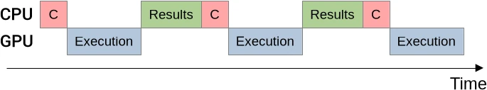
…where “C” stands for command buffer recording, “Execution” stands for execution of GPU work (simulation + results downloads) and “Results” stands for CPU-side results processing.

Command buffer recording has been purposely abbreviated on this diagram as it is expected to be faster than the other two steps, whose relative performance will depends on runtime configuration (relative speed of the GPU and storage device, number of simulation steps per output image…).

In this chapter, we will see how we can make more of these steps happen in parallel.

Command recording

Theory

Because command recording is fast with respect to command execution, allowing them to happen in parallel is not going to save much time. But it will be an occasion to introduce some optimization techniques, that we will later apply on a larger scale to achieve the more ambitious goal of overlapping GPU operations with CPU result processing.

First of all, by looking back at the main simulation loop above, it should be clear to you that it is not possible for the recording of the first command buffer to happen in parallel with its execution. We cannot execute a command buffer that it is still in the process of being recorded.

What we can do, however, is change the logic of our main simulation loop after this first command buffer has been submitted to the GPU:

• Instead of immediately waiting for the GPU to finish the freshly submitted work, we can start preparing a second command buffer on the CPU side while the GPU is busy working on the first command buffer that we just sent.
• Once that second command buffer is ready, we have nothing else to do on the CPU side (for now), so we will just finish executing our first main loop iteration as before: await GPU execution, then process results.
• By the time we reach the second main loop iteration, we will be able to reap the benefits of our optimization by having a second command buffer that can be submitted right away.
• And then the cycle will repeat: we will prepare the command buffer for the third main loop iteration while the GPU work associated with the second main loop iteration is executing, then we will wait, process the second GPU result, and so on.

This sort of ahead-of-time command buffer preparation will result in parallel CPU/GPU execution through pipelining, a general-purpose optimization technique that can improve execution speed at the expense of some duplicated resource allocation and reduced code clarity.

In this particular case, the resource that is being duplicated is the command buffer. Before we used to have only one command buffer in flight at any point in time. Now we intermittently have two of them, one that is being recorded while another one is executing.

And in exchange for this resource duplication, we expect to get a new execution timeline…

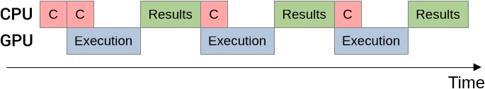
…where command buffer recording and GPU work execution can run in parallel as long as the simulation produces at least two images, resulting in a small performance gain.

Implementation

The design of the SimulationRunner, introduced in the previous chapter, allows us to implement this pipelining optimization through a small modification of our run_simulation() main loop:

// Prepare the first command buffer
let mut cmdbuf = Some(runner.schedule_next_output()?);

// Produce the requested amount of concentration tables
let num_output_images = options.num_output_images;
for image_idx in 0..num_output_images {
    // Submit the command buffer to the GPU and prepare to wait for it
    let future = cmdbuf
        .take()
        .expect("if this iteration executes, a command buffer should be present")
        .execute(context.queue.clone())?
        .then_signal_fence_and_flush()?;

    // Prepare the next command buffer, if any
    if image_idx != num_output_images - 1 {
        cmdbuf = Some(runner.schedule_next_output()?);
    }

    // Wait for the GPU to be done
    future.wait(None)?;

    // Process the simulation output, if enabled
    runner.process_output()?;
}

How does this work?

• Before we begin the main simulation loop, we initialize the simulation pipeline by building a first command buffer, which we do not submit to the GPU right away.
• On each simulation loop iteration, we submit a previously prepared command buffer to the GPU. But in contrast with our previous logic, we do not wait for it right away. Instead, we prepare the next command buffer (if any) while the GPU is executing work.
• Submitting a command buffer to the GPU moves it away, and the static analysis within the Rust compiler that detects use-after-move is unfortunately too simple to understand that we are always going to put another command buffer in its place before the next loop iteration, if there is a next loop iteration. We must therefore play a little trick with the Option type in order to convince the compiler that our code is correct:
  • At first, we wrap our initial command buffer into Some(), thus turning what was an Arc<PrimaryAutoCommandBuffer> into an Option<Arc<PrimaryAutoCommandBuffer>>.
  • When the time comes to submit a command buffer to the GPU, we use the take() method of the Option type to retrieve our command buffer, leaving a None in its place.
  • We then use expect() on the resulting Option to assert that we know it previously contained a command buffer, rather than a None.
  • Finally, when we know that there is going to be a next loop iteration, we prepare the associated command buffer and put it back in the cmdbuf option variable.

While this trick may sound expensive from a performance perspective, you must understand that…

• The Rust compiler’s LLVM backend is a bit more clever than its use-after-move detector, and therefore likely to figure this out and optimize out the Option checks.
• Even if LLVM does not manage, it is quite unlikely that the overhead of checking a boolean flag (testing if an Option is Some) will have any meaningful performance impact compared to the surrounding overhead of scheduling GPU work.

Conclusion

After this coding interlude, we are ready to reach some preliminary conclusions:

• Pipelining is an optimization that can be applied when a computation has two steps A and B that execute on different hardware, and step A produces an output that step B consumes.
• Pipelining allows you to run steps A and B in parallel, at the expense of…
  • Needing to juggle with multiple copies of the output of step A (which will typically come at the expense of a higher application memory footprint).
  • Having a more complex initialization procedure before your main loop, in order to bring your pipeline to the fully initialized state that your main loop expects.
  • Needing some extra logic to avoid unnecessary work at the end of the main loop, if you have real-world use cases where the number of main loop iterations is small enough that this extra work has measurable overhead.

As for performance benefits, you have been warned at the beginning of this section that command buffer recording is only pipelined here because it gives you an easy introduction to this pipelining, and not because the author considers it to be worthwhile.

And indeed, even in a best-case microbenchmarking scenario, the asymptotic performance benefit will be below our performance measurements’ sensitivity threshold…

run_simulation/workgroup16x16/domain2048x1024/total512/image1/compute
                        time:   [136.74 ms 137.80 ms 138.91 ms]
                        thrpt:  [7.7300 Gelem/s 7.7921 Gelem/s 7.8527 Gelem/s]
                 change:
                        time:   [-3.2317% -1.4858% +0.3899%] (p = 0.15 > 0.05)
                        thrpt:  [-0.3884% +1.5082% +3.3396%] No change in
                        performance detected.

Still, this pipelining optimization does not harm much either, and serves as a gateway to more advanced ones. So we will keep it for now.

Results processing

Theory

Encouraged by the modest but tangible performance improvements that pipelined command buffer recording brought, you may now try to achieve full CPU/GPU execution pipelining, in which GPU-side work execution and CPU-side results processing can overlap…

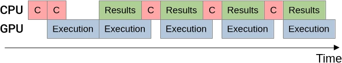
…but your first attempt will likely end with a puzzling compile-time or run-time error, which you will stare at blankly for a few minutes of incomprehension, before you figure it out and thank rustc or vulkano for saving you from yourself.

Indeed there is a trap with this form of pipelining, and one that is easy to fall into: if you are not careful, you are likely to end up trying to access a simulation result on the CPU side, that the GPU could be simultaneously overwriting with a newer result at the same time. Which is the textbook example of a variety of undefined behavior known as a data race.

To avoid this data race, we will need to add double buffering to our CPU-side VBuffer abstraction¹, so that our CPU code can read result N at the same time as our GPU code is busy producing result N+1 and transferring it to the CPU side. And the logic behind our main simulation loop is going to become a bit more complicated again, as we now need to…

• Make sure that by the time we enter the main simulation loop, a result is already available or in the process of being produced. Indeed, the clearest way to write pipelined code is to write each iteration of our main loop under the assumption that the pipeline is already operating at full capacity, taking any required initialization step to get there before the looping begins.
• Rethink our CPU-GPU synchronization strategy so that the CPU code waits for a GPU result to be available before processing it, but does not start processing a result before having scheduled the production of the next result.

Double-buffered VBuffer

As mentioned above, we are going to need some double-buffering inside of VBuffer, which we are therefore going to rename to VBuffers. By now, you should be familiar with the basics of this pattern: we duplicate data storage and add a data member whose purpose is to track the respective role of each of our two buffers…

/// CPU-accessible double buffer used to download the V species' concentration
pub struct VBuffers {
    /// Buffers in which GPU data will be downloaded
    buffers: [Subbuffer<[Float]>; 2],

    /// Truth the the second buffer of the `buffers` array should be used
    /// for the next GPU-to-CPU download
    current_is_1: bool,

    /// Number of columns in the 2D concentration table, including zero padding
    padded_cols: usize,
}
//
impl VBuffers {
    /// Set up `VBuffers`
    pub fn new(options: &RunnerOptions, context: &Context) -> Result<Self> {
        use vulkano::memory::allocator::MemoryTypeFilter as MTFilter;
        let padded_rows = padded(options.num_rows);
        let padded_cols = padded(options.num_cols);
        let new_buffer = || {
            Buffer::new_slice(
                context.mem_allocator.clone(),
                BufferCreateInfo {
                    usage: BufferUsage::TRANSFER_DST,
                    ..Default::default()
                },
                AllocationCreateInfo {
                    memory_type_filter: MTFilter::PREFER_HOST | MTFilter::HOST_RANDOM_ACCESS,
                    ..Default::default()
                },
                (padded_rows * padded_cols) as DeviceSize,
            )
        };
        Ok(Self {
            buffers: [new_buffer()?, new_buffer()?],
            padded_cols,
            current_is_1: false,
        })
    }

    /// Buffer where data has been downloaded two
    /// [`schedule_download_and_flip()`] calls ago, and where data will be
    /// downloaded again on the next [`schedule_download_and_flip()`] call.
    ///
    /// [`schedule_download_and_flip()`]: Self::schedule_download_and_flip
    fn current_buffer(&self) -> &Subbuffer<[Float]> {
        &self.buffers[self.current_is_1 as usize]
    }

    // [ ... more methods coming up ... ]
}

…and then we need to think about when we should alternate between our two buffers. As a reminder, back when it contained a single buffer, the VBuffer type exposed two methods:

• schedule_download(), which prepared a GPU command whose purpose is to transfer the current GPU V concentration input to the VBuffer.
• process(), which was called after the previous command was done executing, and took care of executing CPU post-processing work.

Between the points where these two methods are called, a VBuffer could be not used because it was in the process of being overwritten by the GPU. Which, if we transpose this to our new double-buffered design, sounds like a good point to flip the roles of our two buffers: while the GPU is busy writing to one of the internal buffers, we can do something else with the other buffer:

impl VBuffers {
    [ ... ]

    /// Schedule a download of some [`Concentrations`]' current V input into
    /// [`current_buffer()`](Self::current_buffer), then switch to the other
    /// internal buffer.
    ///
    /// Intended usage is...
    ///
    /// - Schedule two simulation updates and output downloads,
    ///   keeping around the associated futures F1 and F2
    /// - Wait for the first update+download future F1
    /// - Process results on the CPU using [`process()`](Self::process)
    /// - Schedule the next update+download, yielding a future F3
    /// - Wait for F2, process results, schedule F4, etc
    pub fn schedule_download_and_flip(
        &mut self,
        source: &Concentrations,
        cmdbuild: &mut CommandBufferBuilder,
    ) -> Result<()> {
        cmdbuild.copy_buffer(CopyBufferInfo::buffers(
            source.current_inout().input_v.clone(),
            self.current_buffer().clone(),
        ))?;
        self.current_is_1 = !self.current_is_1;
        Ok(())
    }

    [ ... ]
}

As the doc comment indicates, we can use schedule_download_and_flip() method as follows…

1. Schedule a first and second GPU update in short succession
   • Both buffers are now in use by the GPU
   • current_buffer() points to the buffer V1 that is undergoing the first GPU update and will be ready for CPU processing first.
2. Wait for the first GPU update to finish.
   • Cuffent buffer V1 is now ready for CPU readout.
   • Buffer V2 is still being processed by the GPU.
3. Perform CPU-side processing on the current buffer V1.
4. We don’t need V1 anymore after this is done, so schedule a third GPU update.
   • current_buffer() now points to buffer V2, which is still undergoing the second GPU update we scheduled.
   • Buffer V1 is now being processed by the third GPU update.
5. Wait for the second GPU update to finish.
   • Current buffer V2 is now ready for CPU readout.
   • Buffer V1 is still being processed by the third GPU update.
6. We are now back at step 3 but with the roles of V1 and V2 reversed. Repeat steps 3 to 5, reversing the roles of V1 and V2 each time, until all desired outputs have been produced.

…which means that the logic of process() function will basically not change, aside from the fact that it will now use the current_buffer() instead of the former single internal buffer:

impl VBuffers {
    [ ... ]

    /// Process the latest download of the V species' concentrations
    ///
    /// See [`schedule_download_and_flip()`] for intended usage.
    ///
    /// [`schedule_download_and_flip()`]: Self::schedule_download_and_flip
    pub fn process(&self, callback: impl FnOnce(ArrayView2<Float>) -> Result<()>) -> Result<()> {
        // Access the underlying dataset as a 1D slice
        let read_guard = self.current_buffer().read()?;

        // Create an ArrayView2 that covers the whole data, padding included
        let padded_cols = self.padded_cols;
        let padded_elements = read_guard.len();
        assert_eq!(padded_elements % padded_cols, 0);
        let padded_rows = padded_elements / padded_cols;
        let padded_view = ArrayView::from_shape([padded_rows, padded_cols], &read_guard)?;

        // Extract the central region of padded_view, excluding padding
        let data_view = padded_view.slice(s!(
            PADDING_PER_SIDE..(padded_rows - PADDING_PER_SIDE),
            PADDING_PER_SIDE..(padded_cols - PADDING_PER_SIDE),
        ));

        // We are now ready to run the user callback
        callback(data_view)
    }
}

Simulation runner changes

Within the implementation of SimulationRunner, our OutputHandler struct which governs simulation output downloads must now be updated to contain VBuffers instead of a VBuffer…

/// State associated with output downloads and post-processing, if enabled
struct OutputHandler<ProcessV> {
    /// CPU-accessible location to which GPU outputs should be downloaded
    v_buffers: VBuffers,

    /// User-defined post-processing logic for this CPU data
    process_v: ProcessV,
}

…and the SimulationRunner::new() constructor of must be adjusted accordingly.

impl<'run_simulation, ProcessV> SimulationRunner<'run_simulation, ProcessV>
where
    ProcessV: FnMut(ArrayView2<Float>) -> Result<()>,
{
    /// Set up the simulation
    fn new(
        options: &'run_simulation RunnerOptions,
        context: &'run_simulation Context,
        process_v: Option<ProcessV>,
    ) -> Result<Self> {
        // [ ... ]

        // Set up the logic for post-processing V concentration, if enabled
        let output_handler = if let Some(process_v) = process_v {
            Some(OutputHandler {
                v_buffers: VBuffers::new(options, context)?,
                process_v,
            })
        } else {
            None
        };

        // [ ... ]
    }

    // [ ... ]
}

But that is the easy part. The slightly harder part is that in order to achieved the desired degree of pipelining, we should revise the responsibility of the scheduler_download_and_flip() method so that instead of simply building a command buffer, it also submits it to the GPU for eager execution:

impl<'run_simulation, ProcessV> SimulationRunner<'run_simulation, ProcessV>
where
    ProcessV: FnMut(ArrayView2<Float>) -> Result<()>,
{
    // [ ... ]

    /// Submit a GPU job that will produce the next simulation output
    fn schedule_next_output(&mut self) -> Result<FenceSignalFuture<impl GpuFuture + 'static>> {
        // Schedule a number of simulation steps
        schedule_simulation(
            self.options,
            &self.pipelines,
            &mut self.concentrations,
            &mut self.cmdbuild,
        )?;

        // Schedule a download of the resulting V concentration, if enabled
        if let Some(handler) = &mut self.output_handler {
            handler
                .v_buffers
                .schedule_download_and_flip(&self.concentrations, &mut self.cmdbuild)?;
        }

        // Extract the old command buffer builder, replacing it with a blank one
        let old_cmdbuild =
            std::mem::replace(&mut self.cmdbuild, command_buffer_builder(self.context)?);

        // Build the command buffer and submit it to the GPU
        let future = old_cmdbuild
            .build()?
            .execute(self.context.queue.clone())?
            .then_signal_fence_and_flush()?;
        Ok(future)
    }

    // [ ... ]
}

…and being nice people, we should also warn users of the process_output() that although its implementation has not changed much, its usage contract has become more complicated:

impl<'run_simulation, ProcessV> SimulationRunner<'run_simulation, ProcessV>
where
    ProcessV: FnMut(ArrayView2<Float>) -> Result<()>,
{
    // [ ... ]

    /// Process the simulation output, if enabled
    ///
    /// This method is meant to be used in the following way:
    ///
    /// - Initialize the simulation pipeline by submitting two simulation jobs
    ///   using [`schedule_next_output()`](Self::schedule_next_output)
    /// - Wait the first simulation job to finish executing
    /// - Call this method to process the output of the first job
    /// - Submit a third simulation job
    /// - Wait the second simulation job to finish executing
    /// - Call this method to process the output of the second job
    /// - ...and so on, until all simulation outputs have been processed...
    fn process_output(&mut self) -> Result<()> {
        if let Some(handler) = &mut self.output_handler {
            handler.v_buffers.process(&mut handler.process_v)?;
        }
        Ok(())
    }
}

Once this is done, migrating run_simulation() to the new pipelined logic becomes straightforward:

/// Simulation runner, with a user-specified output processing function
pub fn run_simulation<ProcessV: FnMut(ArrayView2<Float>) -> Result<()>>(
    options: &RunnerOptions,
    context: &Context,
    process_v: Option<ProcessV>,
) -> Result<()> {
    // Set up the simulation
    let mut runner = SimulationRunner::new(options, context, process_v)?;

    // Schedule the first simulation update
    let mut current_future = Some(runner.schedule_next_output()?);

    // Produce the requested amount of concentration tables
    let num_output_images = options.num_output_images;
    for image_idx in 0..num_output_images {
        // Schedule the next simulation update, if any
        let next_future = (image_idx < num_output_images - 1)
            .then(|| runner.schedule_next_output())
            .transpose()?;

        // Wait for the GPU to be done with the previous update
        current_future
            .expect("if this loop iteration executes, a future should be present")
            .wait(None)?;
        current_future = next_future;

        // Process the simulation output, if enabled
        runner.process_output()?;
    }
    Ok(())
}

As previously hinted, this is quite similar to the previosu logic where we used to prepare a new command buffer while the previous command buffer is executing, except now we take it further and submit a full GPU job while another full GPU job is already executing.

And as before, some tricks must be played with Option in order to convince the Rust compiler’s borrow checker that even though we do not schedule a new computation on the last loop iteration, our inner Option of FenceSignalFuture will always be Some() or we’ll die at runtime, and therefore use-after-move of GPU futures cannot happen.

Exercise

Implement the pipelining techniques described above, then adapt the simulation executable and benchmark, and check the impact on performance.

You should observe a noticeable performance improvement when running the main simulation binary over a fast storage device like /dev/shm, as the previous version of the simulation spent too much time keeping waiting for the GPU to keep this storage device busy.

Microbenchmarks will see more modest performance improvements except for compute+download+sum, which will see a great improvement in scenarios that produce many concentration tables because its CPU post-processing can now run in parallel with GPU work.

1. Another example of how pipelining requires duplication of (in this case memory) resources. ↩