Pipelines

Unlike the GPU context building code, which is rather generic, our previous GPU pipeline was specific to the number-squaring task at hand. So it will take quite a few changes to our pipeline-building procedure before we get to a working Gray-Scott reaction simulation.

Code module

To avoid making our code too complicated for Rust beginners, we will not attempt to fully deduplicate pipeline setup code between the number-squaring and Gray-Scott computations.

Instead, we will create a new dedicated pipeline code module inside of our grayscott module, within which we will copy and paste relevant code from the square pipeline as appropriate.

This can be done by going through the following steps:

• Add a pub mod pipeline item to the exercises/src/grayscott/mod.rs file, which represents the root of the Gray-Scott reaction specific code.
• Create an exercises/src/grayscott/pipeline.rs empty file file inside of this directory, which will host compute pipeline handling code.

Common GLSL infrastructure

Data interface

After the mandatory GLSL version declaration…

#version 460

…we need to think a bit about what our CPU-GPU data interface is going to look like.

• We want to have two input buffers, from which we are going to read data representing the initial concentration of the U and V chemical species.
• We want to have two output buffers, into which we are going to write updated values of the chemical species concentrations.
• These 4 buffers will always be re-bound together (initially in an alternating pattern), and can thus be grouped into a single descriptor set for efficiency.

This data interface is well expressed by the following GLSL code…

// Input and output data buffers
layout(set = 0, binding = 0) restrict readonly buffer InputBuffer {
    float[] data;
} Input[2];
layout(set = 0, binding = 1) restrict writeonly buffer OutputBuffer {
    float[] data;
} Output[2];

// Indexing convention for Input and Output arrays
const uint U = 0;
const uint V = 1;

…which leverages a few new GLSL features that we have not used so far:

• Like C pointers, GLSL data interfaces can be annotated with the restrict keyword. This allows the compiler to assume that they are the only way to read or write the data of interest, resulting in improved optimizations when matters like SIMD get involved (which is the case on all GPU hardware in common use).
• GLSL replaces the C/++ const notion with a more symmetrical scheme based on read and write access. In particular, we can declare buffers as readonly and writeonly when that is our intent, to make sure that using them otherwise becomes a compilation error.
• Because GLSL inherits the C/++ struct limitation of only allowing one flexible array member at the end of a shader storage block, we cannot e.g. model our inputs as a buffer containing both float[] u; and float[] v;. We resolve this with arrays of storage blocks, coupled with helpful consts that let us tell which index of these array represents which chemical species.
  • “But”, you may say, “didn’t you just say that GLSL does not have C-style const?”. Indeed, that is the case. The const keyword in GLSL is for compilation constants that are inlined at the point of use, like const in Rust and static constexpr in C++.

Specialization constants

Now, if you remember the previous example of GLSL code that we have gone through, you will know that we will also want a set of specialization constants, for two different reasons:

• It improves code maintainability by reducing the volume of information that we need to duplicate on the CPU and GPU side of the interface. Such duplication creates a risk that information goes out of sync as we modify either side, resulting in tricky program bugs.
• It allows us to configure the GPU code from the CPU side right at the time where the GPU code is compiled (at application startup time), and thus allows us to…
  1. Avoid run-time configuration, which is a little more cumbersome in Vulkan than in other GPU APIs because the underlying evil hardware mechanics are not hidden.
  2. Benefit from compiler optimizations that leverage knowledge of all application parameters, so that our GPU code gets specialized for this set of parameters.

What specialization constants are we going to need then?

• As before, we will want to have a way to set the execution workgroup size. And because our problem is now two-dimensional, we will want to allow two-dimensional workgroups in addition to one-dimensional ones, as those may come in handy.
• Vulkan storage buffers are one-dimensional,¹ so right now we only know the total number elements of our 2D chemical species tables, and not their aspect ratio. We’ll need this information to correctly perform our stencil computation, so if we don’t hardcode it into the shader, we’ll need to pass it from the CPU side to the GPU side somehow.
• Our computation has a number of parameters that are known either at Rust code compilation time or at GPU pipeline building time, which from the perspective of GPU programming makes no difference. Specialization constants can also be used to pass such constants to the GPU compiler for the sake of making it know as much as possible.

We can encode this set of specializations in GLSL as follows:

// Configurable workgroup size, as before
layout(local_size_x = 8, local_size_y = 8) in;
layout(local_size_x_id = 0, local_size_y_id = 1) in;

// Concentration table width
layout(constant_id = 2) const uint UV_WIDTH = 1920;

// "Scalar" simulation parameters
layout(constant_id = 3) const float FEED_RATE = 0.014;
layout(constant_id = 4) const float KILL_RATE = 0.054;
layout(constant_id = 5) const float DELTA_T = 1.0;

// 3x3 Laplacian stencil
//
// Unfortunately, SPIR-V does not sûpport setting matrices via specialization
// constants at this point in time, so we'll need to hack our way into this
layout(constant_id = 6) const float STENCIL_WEIGHT_11 = 0.25;
layout(constant_id = 7) const float STENCIL_WEIGHT_12 = 0.5;
layout(constant_id = 8) const float STENCIL_WEIGHT_13 = 0.25;
layout(constant_id = 9) const float STENCIL_WEIGHT_21 = 0.5;
layout(constant_id = 10) const float STENCIL_WEIGHT_22 = 0.0;
layout(constant_id = 11) const float STENCIL_WEIGHT_23 = 0.5;
layout(constant_id = 12) const float STENCIL_WEIGHT_31 = 0.25;
layout(constant_id = 13) const float STENCIL_WEIGHT_32 = 0.5;
layout(constant_id = 14) const float STENCIL_WEIGHT_33 = 0.25;
//
// This function call will be inlined by any competent GPU compiler and
// will therefore not introduce any run-time overhead
mat3 stencil_weights() {
    return mat3(
        // CAUTION: GLSL matrix constructors are column-major, which is the
        //          opposite of the convention used by Rust and C/++. Let's make
        //          the life of our CPU code easier by having it provide
        //          specialization constants using its standard convention,
        //          then performing the transpose inside of the GPU compiler.
        vec3(STENCIL_WEIGHT_11, STENCIL_WEIGHT_21, STENCIL_WEIGHT_31),
        vec3(STENCIL_WEIGHT_12, STENCIL_WEIGHT_22, STENCIL_WEIGHT_32),
        vec3(STENCIL_WEIGHT_13, STENCIL_WEIGHT_23, STENCIL_WEIGHT_33)
    );
}

// Finally, the DIFFUSION_RATE constants are best exposed as a vector, following
// our general design of treating (U, V) pairs as arrays or vectors of size 2
layout(constant_id = 15) const float DIFFUSION_RATE_U = 0.1;
layout(constant_id = 16) const float DIFFUSION_RATE_V = 0.05;
//
vec2 diffusion_rate() {
    return vec2(DIFFUSION_RATE_U, DIFFUSION_RATE_V);
}

By now, you should hopefully agree with the author that manually numbering specialization constants like this is error-prone, and something that machines should be doing automatically instead of leaving it up to manual human work. But sadly, the author knows of no way around it today. Hopefully future GPU languages or vulkano updades will improve upon those pesky GLSL binding number ergonomics someday…

Data layout

At this point, we have our CPU/GPU interface fully specified, and can start writing some GPU compute shaders that our CPU code can later call into.

Notice the plural above. For this simulation, we will do a few things differently from before, so that you can get exposed of a few more ways to perform common tasks in Vulkan. Compared to the previous square example, one thing that we are going to do differently is to use two compute shaders instead of one:

• One compute shader, which we will call init, will be used to initialize the U and V arrays directly on the GPU. This way we won’t need to set up expensive CPU-to-GPU transfers just to get a basic initial data pattern that can easily be GPU-generated.
• After this is done, another compute shader, which we will call main, will be repeatedly used to perform the desired amount of Gray-Scott simulation steps.

We will also use a different approach to handling stencil edges. Instead of handling these via irregularly shaped input data windows (with smaller windows on the edges of the simulation domain), as we did at the start of the CPU chapter, we will start with the alternate way of padding the dataset with one line of zeroed values on each edge that encodes boundary conditions.

This approach to edge handling has pros and cons:

• Our code logic will be simpler, which seems good as GPU hardware tends to sacrifice some ability to handle fancy code logic in the name of increased number-crunching poser.
• We will need to be more careful with our data layout computations, adding/subtracting 1 to positions and 2 to storage width/height when appropriate. Basically, there is now a difference between working in the space of the simulated concentration values (inner dark gray rectangle in schematic above) and the space of the actual data storage (outer light gray rectangle), and when we switch between the two in our code we need to perform a coordinate transform.
• We may or may not get memory access alignment issues that can reduce our computational performance on some hardware. If we get them, we can resolve them through clever use of extra unused padding floats. But as GPU hardware is known to be more tolerant of unaligned SIMD accesses than CPU hardware, we will not attempt to resolve this issue unless a GPU profiler tells us that we are having it on some particular hardware of interest.

To handle the “careful layout” part of this tradeoff, we will set up a few GLSL utilities that let us share more code between our two compute shaders, so that at least we only need to write the tricky data layout concern once, and can change more easily change the data layout later if needed:

// Data padding control and handling
const uint PADDING_PER_SIDE = 1;
const uint PADDED_UV_WIDTH = UV_WIDTH + 2 * PADDING_PER_SIDE;
//
// Unlike the above constants, these functions will not be zero cost. However
// all their data inputs are either constant across an entire compute
// dispatch's lifetime (data length()) or compilation constants, so the compiler
// should be able to deduplicate multiple calls to them given enough inlining.
uint padded_uv_height() { return Input[0].data.length() / PADDED_UV_WIDTH; }
uint uv_height() { return padded_uv_height() - 2 * PADDING_PER_SIDE; }

// First/last output position that corresponds to an actual data location and
// not a padding value that should always be zero
const uvec2 DATA_START_POS = uvec2(PADDING_PER_SIDE, PADDING_PER_SIDE);
uvec2 buffer_end_pos() {
    return uvec2(PADDED_UV_WIDTH, padded_uv_height());
}
uvec2 data_end_pos() {
    return buffer_end_pos() - uvec2(PADDING_PER_SIDE);
}

// Convert a 2D location into a linear buffer index
uint pos_to_index(uvec2 pos) {
    return pos.x + pos.y * PADDED_UV_WIDTH;
}

// Read an (U, V) pair from a particular input location
//
// `pos` starts at (0, 0) for the upper-left padding value, with (1, 1)
// corresponding to the first actual data value.
vec2 read(uvec2 pos) {
    uint index = pos_to_index(pos);
    return vec2(
        Input[U].data[index],
        Input[V].data[index]
    );
}

// Write an (U, V) to a particular output location, `pos` works as in `read()`
void write(uvec2 pos, vec2 value) {
    uint index = pos_to_index(pos);
    Output[U].data[index] = value.x;
    Output[V].data[index] = value.y;
}

And that will be it for the code that is shared between our two compute shaders. You can now save all of the above GLSL code, except for the initial #version 460 directive (we’ll get back to this), into a file that at location exercises/src/grayscott/common.comp. And once that is done, we will start writing some actual compute shaders.

Initialization shader

Now that we have some common utilities to interface with our datasets and configure the simulation, let us write out initialization compute shader.

This will mostly be a straightforward GLSL translation of our CPU data initialization code. But because this is GPU code, we need to make a new decision, which is the way GPU work items and workgroups will map onto the work to be done.

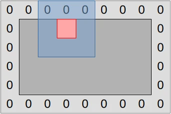
We have decided to go with the simple mapping illustrated by the following schematic:

The CPU command buffer that will eventually execute this compute shader will dispatch enough workgroups (purple squares) to cover the full padded simulation dataset (red zone) with one work item per data point. But work item tasks will vary:

• Padding elements (denoted “0”) will be initialized to zero as they should.
• Non-padding elements (inside the zero padding) will be initialized as in the CPU version.
• Out-of bounds work items (outer purple area) will exit early without doing anything.

This general scheme of having work-items at different position perform different kinds of work will reduce execution efficiency a bit on SIMD GPU hardware, however…

• The impact should be minor at the target dataset size of full HD images (1920x1080 concentration values), where edge elements and out-of-bounds work items should only have a small contribution to the overall execution time.
• The initialization compute shader will only execute once per full simulation run, so unless we have reasons to care about the performance of short simulation runs with very few simulation steps, we should not worry about the performance of this shader that much.

All said and done, we can implement the initialization shader using the following GLSL code:

#version 460

#include "common.comp"

// Polyfill for the standard Rust saturating_sub utility
uint saturating_sub(uint x, uint y) {
    if (x >= y) {
        return x - y;
    } else {
        return 0;
    }
}

// Data initialization entry point
void main() {
    // Map work items into 2D padded buffer, discard out-of-bounds work items
    uvec2 pos = uvec2(gl_GlobalInvocationID.xy);
    if (any(greaterThanEqual(pos, buffer_end_pos()))) {
        return;
    }

    // Fill in zero boundary condition at edge of simulation domain
    if (
        any(lessThan(pos, DATA_START_POS))
        || any(greaterThanEqual(pos, data_end_pos()))
    ) {
        write(pos, vec2(0.0));
        return;
    }

    // Otherwise, replicate standard Gray-Scott pattern in central region
    uvec2 data_pos = pos - DATA_START_POS;
    uvec2 pattern_start = uvec2(
        7 * UV_WIDTH / 16,
        saturating_sub(7 * uv_height() / 16, 4)
    );
    uvec2 pattern_end = uvec2(
        8 * UV_WIDTH / 16,
        saturating_sub(8 * uv_height() / 16, 4)
    );
    bool pattern = all(greaterThanEqual(data_pos, pattern_start))
                   && all(lessThan(data_pos, pattern_end));
    write(pos, vec2(1.0 - float(pattern), float(pattern)));
}

As is customary in this course, we will point out a few things about the above code:

• Like C, GLSL supports #include preprocessor directives that can be used in order to achieve a limited from of software modularity. Here we are using it to make our two compute shaders share a common CPU-GPU interface and a few common utility constants/functions.
• …but for reasons that are not fully clear to the course’s author (dubious GLSL design decision or shaderc compiler bug?), #version directives cannot be extracted into a common GLSL source file and must be present in the source code of each individual compute shader.
• GLSL provides built-in vector and matrix types, which we use here in an attempt to make our 2D computations a little clearer. Use of these types may sometimes be required for performance (especially when small data types like 8-bit integers and half-precision floating point numbers get involved), but here we only use them for expressivity and concision.

To conclude on this part, we will advise that you store the initialization shader provided above into a file at location exercises/src/grayscott/init.comp.

Simulation shader

In the initialization shader that we have just covered, we needed to initialize the entire GPU dataset, padding edges included. And the most obvious way to do this was to map each GPU work item into one position of the full GPU dataset, padding zeroes included.

When it comes to the subsequent Gray-Scott reaction simulation, however, the mapping between work items and data that we should use is less immediately obvious. The two simplest approaches would be to use one work item per input data point (which would include padding, as in our initialization algorithm) or one work item per updated output U/V value (excluding padding). But these approaches entail different tradeoffs:

• Using one work item per input data point allows us to expose a bit more concurrent work to the GPU (one extra work item per padding element), but as mentioned earlier the influence of such edges should be negligible when computing a larger image of size 1920x1080.
• Using one work item per output data point means that each GPU work item can load all of its data inputs without cooperating with other work items, and is the only writer of its data output. But this comes at the expense of each input value being redundantly loaded ≤8 more times by the Laplacian computations associated with all output data points at neighboring 2D positions.
• In contrast, with one work item per input data point, we will perfom no redundant data loading work, but will need to synchronize work items with each other in order to perform the Laplacian computation, because a Laplacian computation’s inputs now come from multiple work items. Synchronization comes at the expense of extra code complexity, and also adds some overhead that may negate the benefits of avoiding redundant memory loads.

Since there is no obviously better approach here, it is best to try both and compare their performance. Therefore, in the initial version of our Gray-Scott GPU implementation we will start with the simplest code of using one work item per output data point, which is illustrated below. And later on, after we get a basic simulation working, we will discuss optimizations that reduce the costs of redundant Laplacian input loading or eliminate such redundant loading entirely.

The following schematic summarizes the resulting execution and data access strategy:

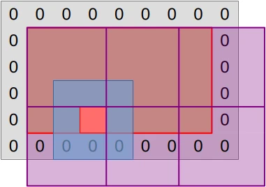
CPU command buffers that will execute the simulation compute shader will dispatch enough workgroups (purple squares) to cover the central region of the simulation dataset (red rectangle) with one work item per data point. Then on the GPU side, work items that map into a padding or out-of-bounds location (purple area) will be ignored and exit early.

Each remaining work item will then proceed to compute the updated (U, V) pair associated with its current location, as illustrated by the concentric blue and red squares:

• The work-item will load the current (U, V) value associated with its assigned location (red square) and all neighboring (U, V) values (blue square) from the input buffers.
• It will then perform computations based one these inputs that will eventually produce an updated (U, V) value, which will be written down to the matching location of the output buffers.

The resulting GLSL code looks like this…

#version 460

#include "common.comp"

// Simulation step entry point
void main() {
    // Map work items into 2D central region, discard out-of-bounds work items
    uvec2 pos = uvec2(gl_GlobalInvocationID.xy) + DATA_START_POS;
    if (any(greaterThanEqual(pos, data_end_pos()))) {
        return;
    }

    // Load central value
    vec2 uv = read(pos);

    // Compute the diffusion gradient for U and V
    uvec2 topleft = pos - uvec2(1);
    mat3 weights = stencil_weights();
    vec2 full_uv = vec2(0.0);
    float sum_weights = 0.0;
    for (int y = 0; y < 3; ++y) {
        for (int x = 0; x < 3; ++x) {
            vec2 stencil_uv = read(topleft + uvec2(x, y));
            float weight = weights[x][y];
            full_uv += weight * stencil_uv;
            sum_weights += weight;
        }
    }
    full_uv -= sum_weights * uv;

    // Deduce the change in U and V concentration
    float u = uv.x;
    float v = uv.y;
    float uv_square = u * v * v;
    vec2 delta_uv = diffusion_rate() * full_uv + vec2(
        FEED_RATE * (1.0 - u) - uv_square,
        uv_square - (FEED_RATE + KILL_RATE) * v
    );
    write(pos, uv + delta_uv * DELTA_T);
}

…and the proposed location for saving it is exercises/src/grayscott/main.comp.

SPIR-V interface

Now that the GLSL is taken care of, it is time to work on the Rust side. Inside of exercises/src/grayscott/pipeline.rs, let’s ask vulkano to build the SPIR-V shader modules and create some Rust-side constants mirroring the GLSL specialization constants as we did before…

//! Gray-Scott simulation compute pipelines

/// Shader module used for compute pipelines
mod shader {
    vulkano_shaders::shader! {
        shaders: {
            init: {
                ty: "compute",
                path: "src/grayscott/init.comp"
            },
            main: {
                ty: "compute",
                path: "src/grayscott/main.comp"
            },
        }
    }
}

/// Descriptor set that is used to bind input and output buffers to the shader
pub const DATA_SET: u32 = 0;

// Descriptor array bindings within DATA_SET, in (U, V) order
pub const IN: u32 = 0;
pub const OUT: u32 = 1;

// === Specialization constants ===
//
// Workgroup size
const WORKGROUP_SIZE_X: u32 = 0;
const WORKGROUP_SIZE_Y: u32 = 1;
//
/// Concentration table width
const UV_WIDTH: u32 = 2;
//
// Scalar simulation parameters
const FEED_RATE: u32 = 3;
const KILL_RATE: u32 = 4;
const DELTA_T: u32 = 5;
//
/// Start of 3x3 Laplacian stencil
const STENCIL_WEIGHT_START: u32 = 6;
//
/// Diffusion rate of U
const DIFFUSION_RATE_U: u32 = 15;
const DIFFUSION_RATE_V: u32 = 16;

…which will save us from the pain of figuring out magic numbers in the code later on.

Notice that in the code above, we use a variation of the default vulkano_shaders syntax, which allows us to build multiple shaders at once. This makes some things more convenient, for example auto-generated Rust structs will be deduplicated, and it is possible to set some vulkano_shaders options once for all the shaders that we are compiling.

Specialization

As before, we will define some CLI options that will let us tune our (now 2D) workgroup size…

// Add CLI args to pipeline.rs...

use clap::Args;
use std::num::NonZeroU32;

/// CLI parameters that guide pipeline creation
#[derive(Debug, Args)]
pub struct PipelineOptions {
    /// Number of rows in a workgroup
    #[arg(short = 'R', long, default_value = "8")]
    pub workgroup_rows: NonZeroU32,

    /// Number of columns in a workgroup
    #[arg(short = 'C', long, default_value = "8")]
    pub workgroup_cols: NonZeroU32,
}

// ...then put them into the overall CLI args in options.rs

use super::pipeline::PipelineOptions;

#[derive(Debug, Parser)]
#[command(version)]
pub struct Options {
    // [ ... after existing members ... ]
    #[command(flatten)]
    pub pipeline: PipelineOptions,
}

…which will then allow us to set all specialization constants from our shader modules:

// Back to pipeline.rs

use super::options::{self, Options, STENCIL_WEIGHTS};
use crate::Result;
use std::sync::Arc;
use vulkano::{
    shader::{ShaderModule, SpecializationConstant, SpecializedShaderModule},
};

/// Set up a specialized shader module with a certain workgroup size
fn setup_shader_module(
    module: Arc<ShaderModule>,
    options: &Options,
) -> Result<Arc<SpecializedShaderModule>> {
    // Set specialization constants. We'll be less careful this time because
    // there are so many of them in this kernel
    let mut constants = module.specialization_constants().clone();
    assert_eq!(
        constants.len(),
        17,
        "Unexpected amount of specialization constants"
    );
    use SpecializationConstant::{F32, U32};
    //
    *constants.get_mut(&WORKGROUP_SIZE_X).unwrap() = U32(options.pipeline.workgroup_cols.get());
    *constants.get_mut(&WORKGROUP_SIZE_Y).unwrap() = U32(options.pipeline.workgroup_rows.get());
    //
    *constants.get_mut(&UV_WIDTH).unwrap() = U32(options.runner.num_cols as _);
    //
    *constants.get_mut(&FEED_RATE).unwrap() = F32(options.update.feedrate);
    *constants.get_mut(&KILL_RATE).unwrap() = F32(options.update.killrate);
    *constants.get_mut(&DELTA_T).unwrap() = F32(options.update.deltat);
    //
    for (offset, weight) in STENCIL_WEIGHTS.into_iter().flatten().enumerate() {
        *constants
            .get_mut(&(STENCIL_WEIGHT_START + offset as u32))
            .unwrap() = F32(weight);
    }
    //
    *constants.get_mut(&DIFFUSION_RATE_U).unwrap() = F32(options::DIFFUSION_RATE_U);
    *constants.get_mut(&DIFFUSION_RATE_V).unwrap() = F32(options::DIFFUSION_RATE_V);

    // Specialize the shader module accordingly
    Ok(module.specialize(constants)?)
}

Careful readers of the square code will notice that the API design here is a little different from what we had before. We used to load the shader module inside of setup_shader_module(), whereas now we ask the caller to load the shader module and pass it down.

The reason for this change is that now we have two different compute shaders to take care of (one initialization shader and one simulation shader), and we will want to perform the same specialization constant work for both of them. And as it turns out, changing the function signature change like this will allow us to do exactly that.

Multiple shaders, single layout

As in the previous square example, our two compute shaders will each have a single entry point. Which means that we can pretty much reuse the previous setup_compute_stage() function:

/// Set up a compute stage from a previously specialized shader module
fn setup_compute_stage(module: Arc<SpecializedShaderModule>) -> PipelineShaderStageCreateInfo {
    let entry_point = module
        .single_entry_point()
        .expect("GLSL compute shader should have a single entry point");
    PipelineShaderStageCreateInfo::new(entry_point)
}

However, if we proceed to do everything else as in the square example, we will end up with two compute pipeline layouts, which means that we will need two versions of each resource descriptor set we create, one per compute pipeline. This sounds a little ugly and wasteful, so we would like to get our two compute pipelines to share a common pipeline layout.

Vulkan supports this by allowing a pipeline’s layout to describe a superset of the resources that the pipeline actually uses. If we consider our current GPU code in the eyes of this rule, this means that a pipeline layout for the main compute shader can also be used with the init compute shader, because the set of resources that init uses (Output storage block) is a subset of the set of resources that main uses (Input and Output storage blocks).

But from a software maintainability perspective, we would rather not hardcode the assumption that the main pipeline will forever use a strict superset of the resources used by all other GPU pipelines, as we might later want to e.g. adjust the definition of init in a manner that uses resources that main doesn’t need. But thankfully we do not have to do this.

The PipelineDescriptorSetLayoutCreateInfo convenience helper from vulkano that we have used earlier is not limited to operating on a single GPU entry point. Its constructor accepts an iterable set of PipelineStageCreateInfo, and if you provide multiple ones it will attempt to produce a pipeline layout that is compatible with all of the underlying entry points by computing the union of their layout requirements.

Obviously, this layout requirements union computation will only work if the the entry points do not have incompatible layout requirement (e.g. one declares that set 0, binding 0 maps into a buffer while the other declares that it is an image). But there is not risk of this happening to us here as both compute shaders share the same CPU-GPU interface specification from common.comp. So we can safely use this vulkano functionality as follows:

use vulkano::{
    descriptor_set::layout::DescriptorType,
    pipeline::layout::{PipelineDescriptorSetLayoutCreateInfo, PipelineLayout},
};

/// Set up the compute pipeline layout
fn setup_pipeline_layout<const N: usize>(
    device: Arc<Device>,
    stages: [&PipelineShaderStageCreateInfo; N],
) -> Result<Arc<PipelineLayout>> {
    // Auto-generate a sensible pipeline layout config
    let layout_info = PipelineDescriptorSetLayoutCreateInfo::from_stages(stages);

    // Check that the pipeline layout meets our expectation
    //
    // Otherwise, the GLSL interface was likely changed without updating the
    // corresponding CPU code, and we just avoided rather unpleasant debugging.
    assert_eq!(
        layout_info.set_layouts.len(),
        1,
        "This program should only use a single descriptor set"
    );
    let set_info = &layout_info.set_layouts[DATA_SET as usize];
    assert_eq!(
        set_info.bindings.len(),
        2,
        "The only descriptor set should only contain a single binding"
    );
    let input_info = set_info
        .bindings
        .get(&IN)
        .expect("An input data binding should be present");
    assert_eq!(
        input_info.descriptor_type,
        DescriptorType::StorageBuffer,
        "The input data binding should be a storage buffer binding"
    );
    assert_eq!(
        input_info.descriptor_count, 2,
        "The input data binding should contain U and V data buffer descriptors"
    );
    let output_info = set_info
        .bindings
        .get(&OUT)
        .expect("An output data binding should be present");
    assert_eq!(
        output_info.descriptor_type,
        DescriptorType::StorageBuffer,
        "The output data binding should be a storage buffer binding"
    );
    assert_eq!(
        output_info.descriptor_count, 2,
        "The output data binding should contain U and V data buffer descriptors"
    );
    assert!(
        layout_info.push_constant_ranges.is_empty(),
        "This program shouldn't be using push constants"
    );

    // Finish building the pipeline layout
    let layout_info = layout_info.into_pipeline_layout_create_info(device.clone())?;
    let layout = PipelineLayout::new(device, layout_info)?;
    Ok(layout)
}

Conclusion & Exercise

We now have all the building blocks that we need in order to build Vulkan compute pipelines for our data-initialization and simulation shaders, with a shared layout that will later allow us to have common descriptor sets for all pipelines. Time to put it all together into a single struct:

use crate::context::Context;
use vulkano::pipeline::compute::ComputePipeline;

/// Initialization and simulation pipelines with common layout information
#[derive(Clone)]
pub struct Pipelines {
    pub init: Arc<ComputePipeline>,
    pub main: Arc<ComputePipeline>,
    pub layout: Arc<PipelineLayout>,
}
//
impl Pipelines {
    // Set up all the compute pipelines
    pub fn new(context: &Context, options: &Options) -> Result<Self> {
        // TODO: Implement all these functions
    }
}

Your goal for this chapter’s exercise will be to take inspiration from the equivalent struct in the number-squaring pipeline that we studied earlier, and use this inspiration implement the new() constructor for our new set of compute pipelines.

Then you will create (for now unused) Pipelines in the main simulation binary (exercises/src/bin/simulate.rs). And after that you will make sure that debug builds of said binary executes without any error or unexpected warning from the Vulkan validation layers.

Finally, if you are a more experienced Rust developer and want to practice your generics a bit, you may also try deduplicating the logic associated with the init and main entry points inside of the Pipelines::new() constructor.

1. Being aware of this major shortcoming of traditional CPU programming, GPUs also support multi-dimensional memory resources backed by specialized texturing hardware, which should provide performance that’s impossible to beat with 1D buffer indexing code. So the author of this course tried to use these… and experienced great disappointment. Ask for the full story. ↩